Introduction to Tensors, TensorFlow Functions and TensorFlow Datasets

In this tutorial, we will learn about some key aspects of TensorFlow. First we will start by discussing tensors, tensorflow’s fundamental data type. Next, we’ll cover tf.function and when to use it for performance optimization and model portability. Lastly we will discuss tf.data.Dataset methods and how to create tensor-formatted datasets for efficient datapipelines that operate on large datasets.

This is an adaptation from Introduction to Tensors, TensorFlow Functions, and tf.data.Dataset API.

import tensorflow as tf
import numpy as np

Basics of tensors

Let’s create some basic tensors.

A tensor is a multi-dimensional array with a consistent type (known as a dtype). All supported dtypes can be seen with tf.dtypes.DType.

Tensors are similar to NumPy np.arrays.

Tensors are immutable, just like Python numbers and strings. The contents of a tensor can never be updated; only new ones can be created.

Note that we will use tf.constant regularly, and sometimes you’ll see tf.variable for similarly looking assignments. The difference between the two in TensorFlow usage is that, the value assigned to a constant cannot be changed in the future; it is static and the initialization is with a value, not an operation. Whereas for variable, the initialization can be a value or an operation, both of which can change. In the context of machine learning, we would want to assign the loss value as a variable as it changes with each epoch, whereas we would want to assign fixed hyper-parameters like batch size as a constant. Training samples (images for example) are also converted to tensors as constants as they don’t change.

Can you guess where else in the machine learning life cycle we would want to use variables instead of constants and vice versa?

Significance of Tensor shapes

A tensor has a shape. Some key terms to know:

• Shape: Describes the number of axes and length (number of elements) in each axis of a tensor.

• Rank: Determined by the number of axes in a tensor.

• Axis or Dimension: A dimension of a tensor.

• Size: The total number of elements in a tensor. This can be expressed as the product of the shape vector’s elements, e.g. a tensor shape of (256, 256, 3) will have a size of 196608.

A “scalar” is a “rank-0” tensor. It contains a single value and no “axes”.

# This will be an int32 tensor by default; see "dtypes" below.
rank_0_tensor = tf.constant(4)
print(rank_0_tensor)

A “vector” is a “rank-1” tensor and contains something like a list of values.

# Let's make this a float tensor.
rank_1_tensor = tf.constant([2.0, 3.0, 4.0])
print(rank_1_tensor)

A “matrix” is a “rank-2” tensor and it has at least two axes. This is what a single channel image turns out to be in tensor format.

# If you want to be specific, you can set the dtype (see below) at creation time
rank_2_tensor = tf.constant([[1, 2],
                             [3, 4],
                             [5, 6]], dtype=tf.float16)
print(rank_2_tensor)

A scalar, shape: []	A vector, shape: [3]	A matrix, shape: [3, 2]

Tensors can feature more axes, as is required for representation of multi-channel images. For example, we can have a tensor with three axes.

# There can be an arbitrary number of
# axes (sometimes called "dimensions")

rank_3_tensor = tf.constant([
  [[0, 1, 2, 3, 4],
   [5, 6, 7, 8, 9]],
  [[10, 11, 12, 13, 14],
   [15, 16, 17, 18, 19]],
  [[20, 21, 22, 23, 24],
   [25, 26, 27, 28, 29]],])

print(rank_3_tensor)

A tensor with more than two axes can be visualized in several ways.

A 3-axis tensor, shape: [3, 2, 5]

# Something like a small 3 channel image

rank_3_tensor = tf.constant([
  [[0, 1, 2, 3, 4],
   [5, 6, 7, 8, 9]],
  [[10, 11, 12, 13, 14],
   [15, 16, 17, 18, 19]],
  [[20, 21, 22, 23, 24],
   [25, 26, 27, 28, 29]],])

print(rank_3_tensor)

Interpreting tensor shapes

tf.TensorShape objects describe some key properties of tensor shapes which help us understand the dimensionality of the data.

rank_4_tensor = tf.zeros([3, 2, 4, 5]) # A fairly complex shape as an example

A rank-4 tensor, shape: [3, 2, 4, 5]

print("Type of every element:", rank_4_tensor.dtype)
print("Number of axes:", rank_4_tensor.ndim)
print("Rank: ", tf.rank(rank_4_tensor))
print("Shape of tensor:", rank_4_tensor.shape)
print("Elements along axis 0 of tensor:", rank_4_tensor.shape[0])
print("Elements along the last axis of tensor:", rank_4_tensor.shape[-1])
print("Total number of elements (3*2*4*5): ", tf.size(rank_4_tensor).numpy())

Axes of a tensor follow a global to local ordering. For example, in machine learning we often talk about batches. For a given batch, the dimension of the batch is ordered first, followed by the batch element’s spatial dimensions (height, width) and then the channels (referred to as features in the below diagram).

Typical axis order

Types of tensors often used

Most tensors we encounter in computer vision contain floats and integers, but tensors can also represent other types, such as:

• complex numbers

• strings

TensorFlow requires a tf.Tensor to be “rectangular,” which means that every element along an axis is the same size. There are exceptions to this (ragged and sparse tensors, but those are more rare).

We can calculate basic mathematical operations on tensors, such as addition, element-wise multiplication, and matrix multiplication.

a = tf.constant([[1, 2],
                 [3, 4]])
b = tf.constant([[1, 1],
                 [1, 1]]) # Could have also said `tf.ones([2,2], dtype=tf.int32)`

print(tf.add(a, b), "\n") # element-wise addition
print(tf.multiply(a, b), "\n") # element-wise multiplication
print(tf.matmul(a, b), "\n") # matrix multiplication

print(a + b, "\n") # element-wise addition
print(a * b, "\n") # element-wise multiplication
print(a @ b, "\n") # matrix multiplication

Tensors are used in many types of operations (or “Ops”), such as common machine learning operations like tf.math.argmax and tf.nn.softmax.

c = tf.constant([[4.0, 5.0], [10.0, 1.0]])

# Find the largest value
print(tf.reduce_max(c))
# Find the index of the largest value
print(tf.math.argmax(c))
# Compute the softmax
print(tf.nn.softmax(c))

NumPy arrays can be created from tensors using either the np.array or tensor.numpy methods:

rank_2_tensor.numpy()

np.array(rank_2_tensor)

Generally, where tensors are expected, TensorFlow functions additionally accept anything that can be converted to a Tensor using tf.convert_to_tensor.

tf.convert_to_tensor([1,2,3]) # List

tf.reduce_max([1,2,3]) # List

tf.reduce_max(np.array([1,2,3])) # NumPy array

Variables

As previously mentioned, normal tf.Tensors are immutable. However, some objects will change over time, like the trainable weights in a machine learning model. We want to store these values, so in order to do that, we need a tensor that can change. Enter the tf.Variable.

var = tf.Variable([0.0, 0.0, 0.0]) # example rank 1 variable

var.assign([1, 2, 3]) # change / re-assign the contents of the variable

var.assign_add([1, 1, 1]) # change the contents of the variable using an operation

Indexing

Single-axis indexing

In TensorFlow, standard Python indexing rules apply. Indexing tensors looks similar to indexing a list in Python. The same applied for NumPy-style indexing.

• indexes begin at 0

• negative indices count backwards from the end

• colons, :, are used for slices: start:stop:step

rank_1_tensor = tf.constant([0, 1, 1, 2, 3, 5, 8, 13, 21, 34])
print(rank_1_tensor.numpy())

When using a scalar to get an element in the tensor, the axis is removed.

print("First:", rank_1_tensor[0].numpy())
print("Second:", rank_1_tensor[1].numpy())
print("Last:", rank_1_tensor[-1].numpy())

When a slice is indexed using : the axis is retained:

print("Everything:", rank_1_tensor[:].numpy())
print("Before 4:", rank_1_tensor[:4].numpy())
print("From 4 to the end:", rank_1_tensor[4:].numpy())
print("From 2, before 7:", rank_1_tensor[2:7].numpy())
print("Every other item:", rank_1_tensor[::2].numpy())
print("Reversed:", rank_1_tensor[::-1].numpy())

Multi-axis indexing

When working with higher ranks of tensors, we may have to use multiple indices.

To do this, we treat each axis independently with the exact same rules as in the single-axis case.

print(rank_2_tensor.numpy())

If we pass an integer for each index for each axis, a scalar is returned.

# Pull out a single value from a 2-rank tensor
print(rank_2_tensor[1, 1].numpy())

We can combine integers and slices when indexing too. This can be useful if, for example, we want a subset of an image.

# Get row and column tensors
print("Second row:", rank_2_tensor[1, :].numpy())
print("Second column:", rank_2_tensor[:, 1].numpy())
print("Last row:", rank_2_tensor[-1, :].numpy())
print("First item in last column:", rank_2_tensor[0, -1].numpy())
print("Skip the first row:")
print(rank_2_tensor[1:, :].numpy(), "\n")

An example for a tensor with 3 axes:

print(rank_3_tensor[:, :, 4])

Selecting the last feature across all locations in each example in the batch

More on how to apply indexing can be found in the tensor slicing guide.

Manipulating tensor shapes

Sometimes, we need to reshape a tensor. For example, we flatten rank 2 tensors to rank 1 when computing things like confusion matrices.

Notes:

• We can reshape a tensor to a new shape so long as it entails the same total number of elements (size).

• Shifting the order of axes is done with tf.transpose instead of tf.reshape.

• You may run across not-fully-specified shapes. Either the shape contains a None (an axis-length is unknown) or the whole shape is None (the rank of the tensor is unknown). This is often useful for machine learning when the images in a batch may have non-uniform width and height dimensions.

# Shape returns a `TensorShape` object that shows the size along each axis
x = tf.constant([[1, 2, 3],
                [4, 5, 6],
                [7, 8, 9]])
print(x.shape)

# Flatten the rank 2 tensor to rank 1 (a vector)
x_flat = tf.reshape(x, [-1])
print(x_flat)

# Shape returns a `TensorShape` object that shows the size along each axis
x = tf.constant([[1], [2], [3]])
print(x.shape)

# You can convert this object into a Python list, too
print(x.shape.as_list())

A tensor can be manipulated into a new shape using the tf.reshape operation.

# You can reshape a tensor to a new shape.
# Note that you're passing in a list
reshaped = tf.reshape(x, [1, 3])

print(x.shape)
print(reshaped.shape)

The original tensor and the newly created one are both held in memory (remember tensors are immutable). TensorFlow abides by C-style “row-major” memory ordering, which means that an increment on the rightmost index corresponds to a single step in memory.

print(rank_3_tensor)

In fact, flattening a tensor shows the order in which it is held in memory.

# A `-1` passed in the `shape` argument says "Whatever fits".
print(tf.reshape(rank_3_tensor, [-1]))

Generally we use tf.reshape to combine or split adjacent axes (or add/remove 1s, similar to np.squeeze).

Taking the below 3x2x5 tensor, we can reshape to (3x2)x5 or 3x(2x5) for example.

print(tf.reshape(rank_3_tensor, [3*2, 5]), "\n")
print(tf.reshape(rank_3_tensor, [3, -1]))

Some good reshapes.

Tensor DTypes

We can find a tf.Tensor’s data type by inspecting the Tensor.dtype property.

Datatypes can be optionally specified when creating a tf.Tensor from a Python object. If left unspecified, TensorFlow inuits and assigns a datatype that can reasonably represent the data. By default, TensorFlow translates Python integers as tf.int32 and Python floating point numbers as tf.float32.

Tensors can be cast to other types.

the_f64_tensor = tf.constant([2.2, 3.3, 4.4], dtype=tf.float64)
the_f16_tensor = tf.cast(the_f64_tensor, dtype=tf.float16)
# Now, cast to an uint8 and lose the decimal precision
the_u8_tensor = tf.cast(the_f16_tensor, dtype=tf.uint8)
print(the_u8_tensor)

Broadcasting

Broadcasting in TensorFlow is based on the equivalent method in NumPy. The premise is that sometimes we need to stretch smaller tensors automatically to fit the size of larger tensors to run combined operations on them.

A simple example is multiplying or adding a tensor to a scalar. The scalar in this case is broadcast to the same shape as the tensor.

x = tf.constant([1, 2, 3])

y = tf.constant(2)
z = tf.constant([2, 2, 2])
# All of these are the same computation
print(tf.multiply(x, 2))
print(x * y)
print(x * z)

Furthermore, tensors with an axis of length 1 can be stretched to match the axis length of another tensor during a combined operation.

As an example, a 3x1 matrix can be element-wise multiplied by a 1x4 matrix to result in a 3x4 matrix. The notation of the axis with length 1 is optional. In other words, the real shape of y is [4].

# These are the same computations
x = tf.reshape(x,[3,1])
y = tf.range(1, 5)
print(x, "\n")
print(y, "\n")
print(tf.multiply(x, y))

A broadcasted add: a [3, 1] times a [1, 4] gives a [3,4]

The same operation without broadcasting looks like this:

x_stretch = tf.constant([[1, 1, 1, 1],
                         [2, 2, 2, 2],
                         [3, 3, 3, 3]])

y_stretch = tf.constant([[1, 2, 3, 4],
                         [1, 2, 3, 4],
                         [1, 2, 3, 4]])

print(x_stretch * y_stretch)  # Again, operator overloading

Broadcasting is usually both time and space efficient, as it never creates the expanded tensors in memory.

The broadcasting operation can be observed with tf.broadcast_to.

print(tf.broadcast_to(tf.constant([1, 2, 3]), [3, 3]))

More on broadcasting can be found in this section of Jake VanderPlas’s book Python Data Science Handbook.

tf.convert_to_tensor

As a reminder, most TensorFlow operations that expect arguments of class tf.Tensor, such as tf.matmul and tf.reshape, will also accept Python objects shaped like tensors.

Under the hood, most TensorFlow ops apply convert_to_tensor to non-tensor arguments, such as NumPy’s ndarray, TensorShape, Python lists, and tf.Variable, all of which will convert automatically.

See the conversion registry tf.register_tensor_conversion_function to know whether a data type will automatically convert.

String tensors

tf.string is a dtype that represents data as strings (variable-length byte arrays) in tensors.

However, string tensors are atomic meaning that they cannot be indexed the way Python strings can. See tf.strings for ways to manipulate them.

An example of a scalar string tensor:

# Tensors can be strings, too here is a scalar string.
scalar_string_tensor = tf.constant("Lima Peru")
print(scalar_string_tensor)

# If you have three string tensors of different lengths, this is OK.
tensor_of_strings = tf.constant(["Lima Peru",
                                 "NASA SERVIR",
                                 "Development Seed"])
# Note that the shape is (3,). The string length is not included.
print(tensor_of_strings)

The b prefix in the above printout indicates that the tf.string dtype is a byte-string, not a unicode string. For more on how to use unicode text in TensorFlow see the Unicode Tutorial.

Also worth noting, unicode characters in TensorFlow are utf-8 encoded.

tf.strings contains some basic string operations, including tf.strings.split.

# You can use split to split a string into a set of tensors
print(tf.strings.split(scalar_string_tensor, sep=" "))

# ...but it turns into a what is known as a `RaggedTensor` if you split up a tensor of strings,
# as each string might be split into a different number of parts.
print(tf.strings.split(tensor_of_strings))

And we also have tf.string.to_number:

text = tf.constant("1 10 100")
print(tf.strings.to_number(tf.strings.split(text, " ")))

In TensorFlow, the tf.string dtype describes all raw bytes data. The tf.io module is used to convert data to and from bytes, as is done when decoding images and parsing text.

Sparse tensors

Data can sometimes be sparse, as might be the case for a wide embedding space. TensorFlow has a data type called tf.sparse.SparseTensor and related operations to support sparse data and work efficiently with it.

A `tf.SparseTensor`, shape: [3, 4]

# Sparse tensors store values by index in a memory-efficient manner
sparse_tensor = tf.sparse.SparseTensor(indices=[[0, 0], [1, 2]],
                                       values=[1, 2],
                                       dense_shape=[3, 4])
print(sparse_tensor, "\n")

# You can convert sparse tensors to dense
print(tf.sparse.to_dense(sparse_tensor))

Functions

In TensorFlow 2, eager execution mode is on by default. This mode enables intuitive use, rapid experimentation and flexibility. However, this mode faces limits with performance and deployability.

tf.function is used to make graphs out of programs. The critical case for it is when we need to build Python-independent dataflow graphs from Python code, with goal of creating performant and portable models. In fact, compiling in tf.function is required to use the SavedModel class.

We will discuss some of the main uses for tf.function.

Before that, it’s worth knowing how and when tf.function is recommended:

1. When you need actually need low-level performance optimizations. Using tf.function to construct your model will assemble a Tensorflow graph, allowing you to execute your computation outside of eager mode more efficiently.

2. When you need to port your model to different runtime environments, like mobile or edge devices.

Debugging is best done in eager mode, then functions from that should be decorated with @tf.function. It’s important to note that a tf.function avoids Python side effects like object mutation or list appends. For example, if you append to a list as a side effect, the append operation will only happen once, when the graph is traced, not every time the graph function is called.

This can be a useful feature if you want to ensure that your function doesn’t have unintended side effects. However, it can also be a source of confusion if you’re expecting Python-style side effects. The best practice is to avoid relying on these Python side effects when using tf.functions, convert python iterables to Tensorflow Datasets, and return any values you need from the function.

Some notes on Keras w.r.t. tf.function:

For machine learning, if you don’t need low-level control of your model training, use the Keras API.

• The Keras API accepts NumPy arrays, Python generators and, tf.data.Datasets.

• It abstracts away the implementation of regularization, activation, and loss calculation, all of which are easily included.

• The Keras API supports tf.distribute to increase the compute efficiency regardless of the hardware configuration.

• It supports arbitrary/custom losses and metrics.

• The Keras API supports callbacks such as tf.keras.callbacks.TensorBoard for enhanced logging and visualization, and also custom callbacks.

• It is easy to use and performant, as it automatically uses TensorFlow graphs under the hood.

Usage

A Function in TensorFlow, (which can be created by adding the @tf.function decorator) behaves like a core TensorFlow operation. It can be executed eagerly.

@tf.function  # The decorator converts `add` into a `Function`.
def add(a, b):
  return a + b

add(tf.ones([2, 2]), tf.ones([2, 2]))  #  [[2., 2.], [2., 2.]]

Functions can be used inside other Functions.

@tf.function
def dense_layer(x, w, b):
  return add(tf.matmul(x, w), b)

dense_layer(tf.ones([3, 2]), tf.ones([2, 2]), tf.ones([2]))

In some cases, Functions are faster than their eager code equivalent. This is especially so for graphs with lots of small ops. However, on the flip side graphs with few expensive ops (like convolutions) may not benefit from much speedup.

import timeit
conv_layer = tf.keras.layers.Conv2D(100, 3)

@tf.function
def conv_fn(image):
  return conv_layer(image)

image = tf.zeros([1, 200, 200, 100])
# Warm up
conv_layer(image); conv_fn(image)
print("Eager conv:", timeit.timeit(lambda: conv_layer(image), number=10))
print("Function conv:", timeit.timeit(lambda: conv_fn(image), number=10))
print("Note how there's not much difference in performance for convolutions")

Use unknown dimensions for flexibility

TensorFlow matches tensors on the basis of their shape. We can use a None dimension as a wildcard to allow Functions to run on variably-sized input. Variably-sized input is frequent when dealing with sequences of different length, or images of different spatial dimensions (sizes) across batches.

@tf.function(input_signature=(tf.TensorSpec(shape=[None], dtype=tf.int32),))  # Note this still works without the arguments
def g(x):
  print(x)
  return x

print(g(tf.constant([1, 2, 3])))
print(g(tf.constant([1, 2, 3, 4, 5])))

Using iterators and generators

TensorFlow has a tf.data.Iterator for iteration. The tf.data API helps implement generator patterns. TensorFlow’s iterators and generators help avoid Python side effects which can surface outside of eager mode.

@tf.function
def buggy_consume_next(iterator):
  tf.print("Value:", next(iterator))

iterator = iter([1, 2, 3])
buggy_consume_next(iterator)
# This reuses the first value from the iterator, rather than consuming the next value.
buggy_consume_next(iterator)
buggy_consume_next(iterator)

@tf.function
def good_consume_next(iterator):
  # This is ok, iterator is a tf.data.Iterator
  tf.print("Value:", next(iterator))

ds = tf.data.Dataset.from_tensor_slices([1, 2, 3])
iterator = iter(ds)
good_consume_next(iterator)
good_consume_next(iterator)
good_consume_next(iterator)

Data

The tf.data.Dataset API represents methods to create tensor-formatted datasets out of many different types of data.

Usage of the API follows the below pattern:

• Create a dataset from your input data.

• Iterate over the dataset, applying any dataset transformations to the data.

Note that iteration occurs through streaming, so it doesn’t matter if a full dataset can’t fit into memory.

The simplest example of creating a dataset is from a python list:

dataset = tf.data.Dataset.from_tensor_slices([1, 2, 3])
for element in dataset:
  print(element)

Transformations: With a dataset, you can use transformations to prepare the data. In machine learning, sometimes we want to augment our data with image flips and rotations for example. Those could be done in the pipeline too.

dataset = tf.data.Dataset.from_tensor_slices([1, 2, 3])
dataset = dataset.map(lambda x: x*2)
list(dataset.as_numpy_iterator())

Common Terms:

• Element: A single result from calling next() on a dataset iterator. Elements are sometimes nested structures containing multiple components.

• Component: The single part in a nested structure of an element.

Supported types:

As nested structures, elements can contain tuples, named tuples, and dictionaries. This is different behavior than that of Python lists. Instead, Python lists require conversion to tensors and then may be treated as components. Element components can express as any type represented in tf.TypeSpec, which includes tf.Tensor, tf.data.Dataset, tf.sparse.SparseTensor, and tf.TensorArray.

import collections
a = 1 # Integer element
b = 2.0 # Float element
c = (1, 2) # Tuple element with 2 components
d = {"a": (2, 2), "b": 3} # Dict element with 3 components
Point = collections.namedtuple("Point", ["x", "y"])
e = Point(1, 2) # Named tuple
f = tf.data.Dataset.range(10) # Dataset element

We can directly read images and labels from np.array format into tf.data.dataset. In the below example, we are creating synthetic 3 channel images and single channel labels with uniform spatial dimensions and subsequently reading them into a dataset using the tf.data.Dataset.from_tensor_slices method. This works if you can fit the NumPy arrays in memory for the images and labels, but if not you’ll need to use a data pipe (example in later tutorial).

image1, image2, image3 = np.zeros((3, 10,10)), np.zeros((3, 10,10)), np.zeros((3, 10,10))
label1, label2, label3 = np.ones((10,10)), np.ones((10,10)), np.ones((10,10))

images = [image1, image2, image3]
labels = [label1, label2, label3]

dataset = tf.data.Dataset.from_tensor_slices((images, labels))
dataset

Data pipelines

We can use the tf.data.Dataset API iterators and generators to construct data pipelines. A data pipeline is used to map a set of processing steps on a large amount of data. With such pipelines, we can stream data iteratively to the same reusable code for processing and have it contribute to the same dataset (e.g. training or validation). As an example, an image data pipeline might involve reading image files from a file system, applying random perturbations or other augmentations to each image, and then randomly shuffling and appending images to a batch for training. In essence, data pipelines built with the tf.data API enable large amounts of data to be read, with support for different data formats, and complex transformations. We will explore a data pipeline in a subsequent lesson, but if you’re curious about data pipelines, you can read more via this guide.

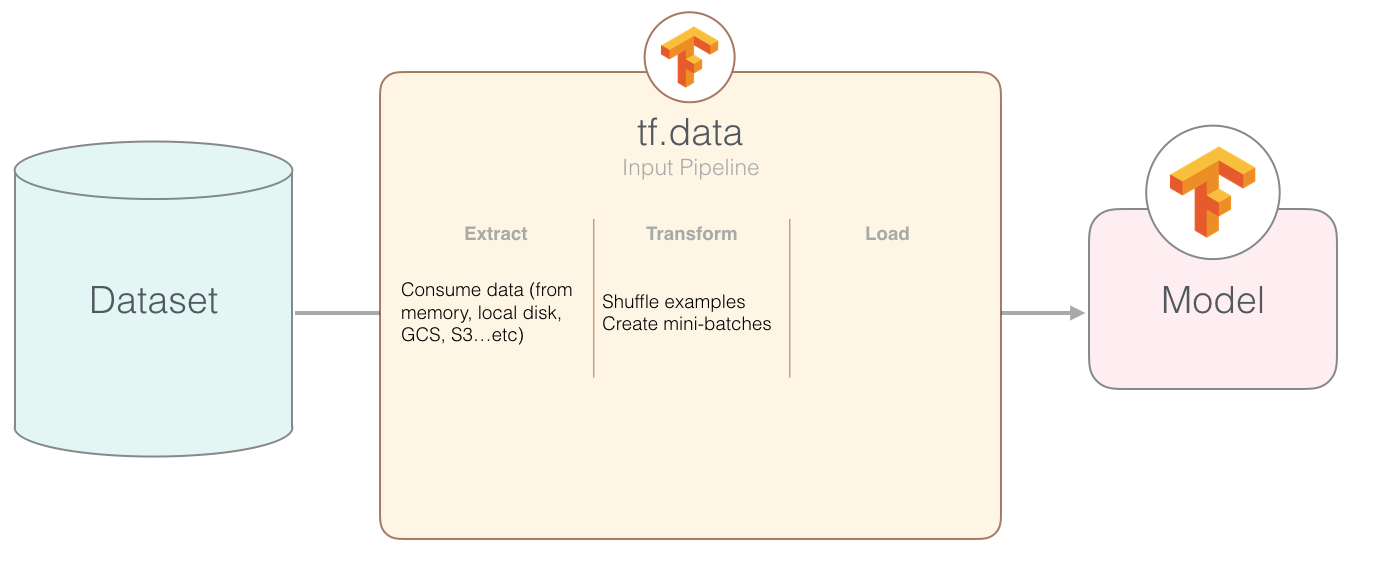
Fig. 22 Figure from Intro to Data Input Pipelines with tf.data

This discussion on datasets is different than the TensorFlow Datasets collection which hosts prepared datasets for TensorFlow models and analysis. We will explore use of the TensorFlow Datasets collection also in other lessons.

#@title Licensed under the Apache License, Version 2.0 (the "License");
# you may not use this file except in compliance with the License.
# You may obtain a copy of the License at
#
# https://www.apache.org/licenses/LICENSE-2.0
#
# Unless required by applicable law or agreed to in writing, software
# distributed under the License is distributed on an "AS IS" BASIS,
# WITHOUT WARRANTIES OR CONDITIONS OF ANY KIND, either express or implied.
# See the License for the specific language governing permissions and
# limitations under the License.