
TensorFlow 2 and Keras quickstart for geospatial computer vision#
This short introduction uses Keras and is adapted from this example.
Our objectives will be to:
Load prebuilt geospatial datasets. We’ll show how to do this firstly with TensorFlow Datasets and secondly with Radiant Earth MLHub.
Build a neural network machine learning model that classifies images.
Train this neural network.
Evaluate the accuracy of the model.
Let’s check the python version we are using. This is subject to Google colab internal updates, so be mindful of when this changes and how that impacts library versions you might be using.
!python3 --version
Python 3.10.12
# install required libraries
!pip install -q rasterio==1.3.8
!pip install -q geopandas==0.13.2
#!pip install -q tensorflow-data-validation==1.3.0 # Only works with Python versions 3.9 or earlier
#!export TFX_DEPENDENCY_SELECTOR=NIGHTLY
#!pip install -q --extra-index-url https://pypi-nightly.tensorflow.org/simple tensorflow-data-validation
!pip install -q radiant_mlhub # for dataset access, see: https://mlhub.earth/
import os, glob, functools, fnmatch, io, shutil, tarfile, json
from zipfile import ZipFile
from itertools import product
from pathlib import Path
import urllib.request
from radiant_mlhub import Dataset, client, get_session, Collection
import pandas as pd
from sklearn.model_selection import train_test_split
from PIL import Image
import numpy as np
from google.colab import drive
import tensorflow_datasets as tfds
from tensorflow.keras.utils import plot_model
#import tensorflow_data_validation
import matplotlib.pyplot as plt
Import TensorFlow into your program to get started:
import tensorflow as tf
print("TensorFlow version:", tf.__version__)
TensorFlow version: 2.13.0
Mount our folders to read and write data.
# set your folders
if 'google.colab' in str(get_ipython()):
    # mount google drive
    drive.mount('/content/gdrive')
    processed_outputs_dir = '/content/gdrive/My Drive/tf-eo-devseed-2-processed-outputs/'
    user_outputs_dir = '/content/gdrive/My Drive/tf-eo-devseed-2-user_outputs_dir'
    if not os.path.exists(user_outputs_dir):
        os.makedirs(user_outputs_dir)
    print('Running on Colab')
else:
    processed_outputs_dir = os.path.abspath("./data/tf-eo-devseed-2-processed-outputs")
    user_outputs_dir = os.path.abspath('./tf-eo-devseed-2-user_outputs_dir')
    if not os.path.exists(user_outputs_dir):
        os.makedirs(user_outputs_dir)
        os.makedirs(processed_outputs_dir)
    print(f'Not running on Colab, data needs to be downloaded locally at {os.path.abspath(processed_outputs_dir)}')
# Move to your user directory in order to write data
%cd $user_outputs_dir
Let’s use a dataset from TensorFlow Datasets#
TensorFlow Datasets, accessible via the importable API tfds, is convenient compared to working with raw geotiffs from file, as the associated pre-packaged datasets are accompanied by TensorFlow’s ecosystem of methods for attribution and exploration. The standardized packaging of these datasets also makes it easier to parallelize pre-processing operations which in turn makes it easier to create simple and efficient data pipelines.
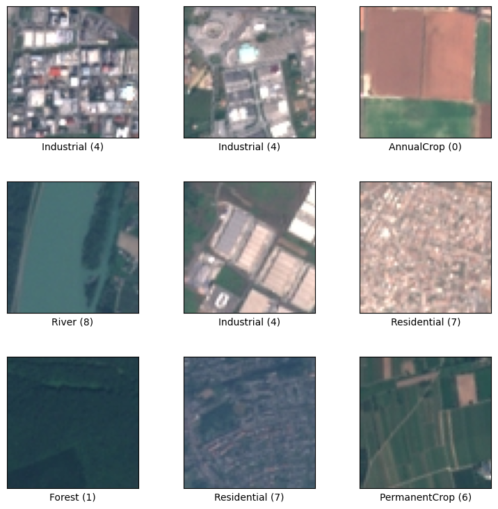
We will use the Eurosat dataset, which contains labeled Sentinel-2 image patches classified into 10 land cover types. More details here: https://www.tensorflow.org/datasets/catalog/eurosat
The classes in this dataset are: ['Industrial', 'Pasture', 'River', 'Forest', 'AnnualCrop', 'PermanentCrop', 'Highway', 'HerbaceousVegetation', 'Residential', 'SeaLake']
The dataset will be partitioned into training, validation and testing splits with a 70:20:10 ratio, respectively.
def convert_datasets(dataset, image_arrays_list, label_integers_list):
  """
  Prepares a dict-style dataset in the format Keras expects, (features, labels).
  """
  for features in dataset.take(len(dataset)):
    image, label = features["image"], features["label"]
    image_arrays_list.append(image)
    label_integers_list.append(label)
  x_dataset, y_dataset = np.array(image_arrays_list), np.array(label_integers_list)
  return x_dataset, y_dataset
# Construct tf.data.Dataset(s)
all_dataset, ds_info = tfds.load(name="eurosat/rgb", split=tfds.Split.TRAIN, with_info=True)

# Shuffle the data before we partition it to make sure we don't have any unwarranted bias
all_dataset = all_dataset.shuffle(1024)
# Extract 30% of samples from the dataset for non-training
val_dataset = all_dataset.take(int(len(all_dataset)*0.3))
# Ensure that 30% of samples is excluded ("skipped") when we set the training dataset
train_dataset = all_dataset.skip(int(len(all_dataset)*0.3))
# Take 30% of the non-training samples to use for testing, this makes up approaximately 10% of the original dataset
test_dataset = val_dataset.take(int(len(val_dataset)*0.3))
# Make sure the validation data skips that test reserve
val_dataset = val_dataset.skip(int(len(val_dataset)*0.3))

print("Number of samples in each split (train, val, test): ", len(train_dataset), len(val_dataset), len(test_dataset))

train_image_arrays = []
train_label_integers = []
val_image_arrays = []
val_label_integers = []
test_image_arrays = []
test_label_integers = []

x_train, y_train = convert_datasets(train_dataset, train_image_arrays, train_label_integers)
x_val, y_val = convert_datasets(val_dataset, val_image_arrays, val_label_integers)
x_test, y_test = convert_datasets(test_dataset, test_image_arrays, test_label_integers)
Number of samples in each split (train, val, test): 18900 5670 2430
# Check for all classes in each split
# set(train_label_integers), set(test_label_integers)
# Dataset specific parameters to be used in the model structure
INPUT_SHAPE =(64, 64, 3)
NUM_CLASSES = 10
Let’s visualize examples of the classes in the dataset
fig = tfds.show_examples(all_dataset, ds_info)
We can also inspect some statistics on the dataset. NOTE: The dependencies for this function are unstable in Python versions >3.9 and may not work as intended under such circumstances.
#tfds.show_statistics(ds_info)
Now, let’s build a very basic machine learning model#
We’ll use the tf.keras.Sequential model structure:
model = tf.keras.models.Sequential([
  tf.keras.layers.Flatten(input_shape=INPUT_SHAPE),
  tf.keras.layers.Dense(128, activation='relu'),
  tf.keras.layers.Dropout(0.2),
  tf.keras.layers.Dense(NUM_CLASSES)
])
The Sequential structure is designed to stack layers where each layer has an input a tensor and an output tensor. Layers themselves are simply functions performing matrix calculations. They may contain trainable variables and are reusable.
It is most common for TensorFlow models to be composed of layers. This sequential model is composed of the Flatten, Dense, and Dropout layers.
For each data sample provided the model, the corresponding output is a vector of logits or log-odds scores, for each class.
predictions = model(x_train[:1]).numpy()
predictions
The tf.nn.softmax function converts logits to probabilities for each class:
tf.nn.softmax(predictions).numpy()
tf.nn.softmax(predictions).numpy().min(), tf.nn.softmax(predictions).numpy().max()
(0.0, 1.0)
The next step is to specify a loss function for training. We will be using losses.SparseCategoricalCrossentropy as it is a commonly used loss function for multi-class data:
loss_fn = tf.keras.losses.SparseCategoricalCrossentropy(from_logits=True)
The input to the loss function is a vector of ground truth values and a vector of logits. The returned output is a scalar loss for each data sample. Loss values close to zero are good, as they imply proximity to the correct class.
The untrained model will produce probabilities close to random for each class.
Before the model can be trained, it needs to be configured and compiled, using Keras Model.compile. In this step, we establish the optimizer class (which in this case will be adam), the loss to the loss_fn function defined earlier, and a metric that will be used evaluate the model at each iteration (herein we will use accuracy).
lr = 0.001 # learning rate
optimizer = tf.keras.optimizers.Adam(learning_rate=lr) # optimizer
model.compile(optimizer=optimizer,
              loss=loss_fn,
              metrics=['accuracy'])
# Summarize the model
model.summary()
Model: "sequential_5"
_________________________________________________________________
 Layer (type)                Output Shape              Param #
=================================================================
 flatten_2 (Flatten)         (None, 12288)             0

 dense_4 (Dense)             (None, 128)               1572992

 dropout_2 (Dropout)         (None, 128)               0

 dense_5 (Dense)             (None, 10)                1290

=================================================================
Total params: 1,574,282
Trainable params: 1,574,282
Non-trainable params: 0
_________________________________________________________________
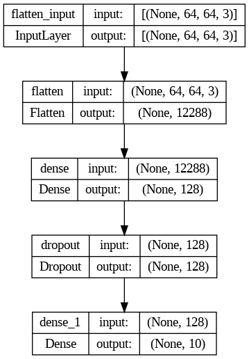
# Visualize the model
plot_model(model, show_shapes=True)
Train and evaluate your model#
No we will train the model using the Model.fit Keras method. During the following iterations, the model parameters will adjust and we will hope to see the loss.
# We will save the model fit history as an object to subsequently get attributes from (e.g. loss curves).
# This is an optional measure.
history = model.fit(x_train, y_train, validation_data= (x_val, y_val), epochs=10)
# plot learning curves
plt.title('Learning Curves')
plt.xlabel('Epoch')
plt.ylabel('Cross Entropy')
plt.plot(history.history['loss'], label='train')
plt.plot(history.history['val_loss'], label='val')
plt.legend()
plt.show()
To evaluate the mode, we will use the Model.evaluate Keras method. The performance is evaluated on a test set.
model.evaluate(x_test, y_test, verbose=2)
We can return probabilities for the predictions by attaching a softmax to the trained model.
probability_model = tf.keras.Sequential([
  model,
  tf.keras.layers.Softmax()
])
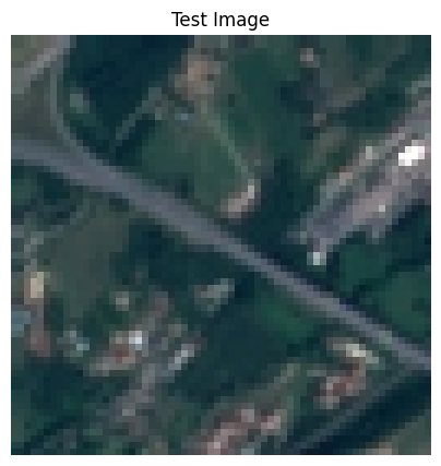
Now, let’s take the first test image, plot it and get the predicted class-wise probabilities.
import matplotlib.pyplot as plt

def display(display_list):
  plt.figure(figsize=(5, 5))

  title = ['Test Image']

  for i in range(len(display_list)):
    plt.subplot(1, len(display_list), i+1)
    plt.title(title[i])
    plt.imshow(tf.keras.preprocessing.image.array_to_img(display_list[i]))
    plt.axis('off')
  plt.show()
# display sample test image
display([x_test[0]])
probabilities = probability_model(x_test[[0]])
probabilities
class_strings = ['Industrial', 'Pasture', 'River', 'Forest', 'AnnualCrop', 'PermanentCrop', 'Highway', 'HerbaceousVegetation', 'Residential', 'SeaLake']
Which class has the highest probability?
for s, p in zip(class_strings, probabilities[0]):
  print(s, p)
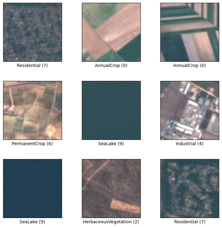
We can look at some ground truth examples again to see if this looks sound!
fig = tfds.show_examples(all_dataset, ds_info)
Part 2 (optional) using same modeling approach but with a dataset from Radiant Earth#
Load and prepare the Drone Imagery Classification Training Dataset for Crop Types in Rwanda dataset from Radiant Earth. You’ll need a Radiant Earth MLHub API key for this.
# configure Radiant Earth MLHub access
!mlhub configure
ds = Dataset.fetch('rti_rwanda_crop_type')
for c in ds.collections:
    print(c.id)
rti_rwanda_crop_type_labels
rti_rwanda_crop_type_source
rti_rwanda_crop_type_raw
collections = [
    'rti_rwanda_crop_type_labels',
    'rti_rwanda_crop_type_source'
]

def download(collection_id):
    print(f'Downloading {collection_id}...')
    collection = Collection.fetch(collection_id)
    path = collection.download('.')
    tar = tarfile.open(path, "r:gz")
    tar.extractall()
    tar.close()
    os.remove(path)

def resolve_path(base, path):
    return Path(os.path.join(base, path)).resolve()

def load_df(collection_id):
    collection = json.load(open(f'{collection_id}/collection.json', 'r'))
    rows = []
    item_links = []
    for link in collection['links']:
        if link['rel'] != 'item':
            continue
        item_links.append(link['href'])
    for item_link in item_links:
        item_path = f'{collection_id}/{item_link}'
        current_path = os.path.dirname(item_path)
        item = json.load(open(item_path, 'r'))
        tile_id = item['id'].split('_')[-1]
        for asset_key, asset in item['assets'].items():
            rows.append([
                tile_id,
                None,
                None,
                asset_key,
                str(resolve_path(current_path, asset['href']))
            ])

        for link in item['links']:
            if link['rel'] != 'source':
                continue
            link_path = resolve_path(current_path, link['href'])
            source_path = os.path.dirname(link_path)
            try:
                source_item = json.load(open(link_path, 'r'))
            except FileNotFoundError:
                continue
            datetime = source_item['properties']['datetime']
            satellite_platform = source_item['collection'].split('_')[-1]
            for asset_key, asset in source_item['assets'].items():
                rows.append([
                    tile_id,
                    datetime,
                    satellite_platform,
                    asset_key,
                    str(resolve_path(source_path, asset['href']))
                ])
    return pd.DataFrame(rows, columns=['tile_id', 'datetime', 'satellite_platform', 'asset', 'file_path'])

for c in collections:
    download(c)

train_df = load_df('rti_rwanda_crop_type_labels')
#test_df = load_df('rti_rwanda_crop_type_labels')
# Read the classes
pd.set_option('display.max_colwidth', None)

data = {'class_names':  ['other', 'banana', 'maize', 'legumes', 'forest', 'structure'],
        'class_ids': [0, 1, 2, 3, 4, 5]
        }

classes = pd.DataFrame(data)
print(classes)

classes.to_csv('rti_rwanda_crop_type_classes.csv')
  class_names  class_ids
0       other          0
1      banana          1
2       maize          2
3     legumes          3
4      forest          4
5   structure          5
train_df_labels = train_df.loc[train_df['asset'] == 'labels']
data_train, data_test = train_test_split(train_df_labels, test_size=0.3, random_state=1)
len(data_train), len(data_test)
(1824, 782)
def get_RE_train_test(dataset, image_array_list, label_integer_list):
  for i, r in data_train.iterrows():
    label_path = r.file_path
    with open(label_path) as f:
      label_obj = json.load(f)
    label_str = label_obj['label']
    label_int = classes.loc[classes['class_names'] == label_str, 'class_ids'].squeeze()
    label_integer_list.append(label_int)
    image_path = label_path.replace('labels', 'source')
    image_path = image_path.replace('source.json', '')
    image_obj = np.array(Image.open(f"{image_path}/image.png"))
    image_array_list.append(image_obj)
  return image_array_list, label_integer_list
train_image_arrays = []
train_label_integers = []

train_image_arrays, train_label_integers = get_RE_train_test(data_train, train_image_arrays, train_label_integers)
test_image_arrays = []
test_label_integers = []

test_image_arrays, test_label_integers = get_RE_train_test(data_test, test_image_arrays, test_label_integers)
set(train_label_integers), set(test_label_integers)
({0, 1, 2, 3, 4, 5}, {0, 1, 2, 3, 4, 5})
x_train, y_train = np.array(train_image_arrays), np.array(train_label_integers)
x_test, y_test = np.array(test_image_arrays), np.array(test_label_integers)
INPUT_SHAPE = (200, 200, 3)
NUM_CLASSES = 6
model = tf.keras.models.Sequential([
  tf.keras.layers.Flatten(input_shape=INPUT_SHAPE),
  tf.keras.layers.Dense(128, activation='relu'),
  tf.keras.layers.Dropout(0.2),
  tf.keras.layers.Dense(NUM_CLASSES)
])

loss_fn = tf.keras.losses.SparseCategoricalCrossentropy(from_logits=True)

model.compile(optimizer='adam',
              loss=loss_fn,
              metrics=['accuracy'])
model.fit(x_train, y_train, epochs=5)
model.evaluate(x_test, y_test, verbose=2)
probability_model = tf.keras.Sequential([
  model,
  tf.keras.layers.Softmax()
])
probability_model(x_test[:5])