Table of Contents
- Data Sourcing
- Data Pipelines
- Data Labeling
- Data Exploration
- Data Versioning
- Data Creation
- Conclusion
Picking up where our Part 1 left off, let’s dive into why we think our open-source ML tooling stack is particularly suited for GeoML, machine learning with earth observation datasets and geospatial labels. To recap, we think the following standards and tools show high potential for a cohesive GeoML stack:
- Datasets and metadata as organized and searchable Spatio Temporal Asset Catalogs (STACs) that are queryable from STAC APIs;
- Traversing STAC Catalogs and querying STAC APIs with pystac_client and materializing the results with stackstac.
- Xarray for the powerful data model that supports subsetting, processing, statistics, and visualization;
- TorchData, Zen3Geo, and Xbatcher as modular and lightweight libraries for streaming geospatial datasets from cloud data stores and converting them into Torch Tensors
- PyTorch and Pytorch Lightning as a set of hierarchical ML frameworks for training ML models for classification, object detection, and segmentation.
In this post we'll focus on the Data Operations section of our ML Tooling chart (which we've updated since Part 1). The following chart lays out tools we‘ve used, evaluated, and liked in green, with tools we are watching in purple.
Fig 1. Our updated ML Tooling diagram, zoomed in on the Data Operations section.
Data Sourcing
How do we access? What API or standard?
The way GeoML data is usually sourced is by downloading it to a hard drive. This can involve assembling geospatial imagery and labels from many disparate sources. For example, a graduate student interested in training a model to detect flooding may download Sentinel-1 source imagery from Copernicus EO Hub -a web-based GUI- extract the vv polarization band, aggregate the data into weekly image composites, then download some labels of flooding sites from a different data portal. At Development Seed, we avoid GUI-based workflows that rely on downloading files. File based workflows aren't readily reproducible, leading to results that are more difficult to test and distribute. Many other organizations are working with scientific data sourced from the cloud, see these great resources from CarbonPlan and Microsoft's AI for Earth program and partner projects for examples.
Files are such a pervasive feature in computing that it seems strange at first to reconsider their use in ML workflows. However, using local files makes reproducibility harder. We want to avoid using files on local disk as much as possible, since local files introduce the complication of paths on one machine being different from paths on another machine.
Instead, we like to access our image datasets via asset links from STAC APIs whenever possible. URLs referencing these STAC APIs are readily shareable and facilitate easy remote dataset access. That means, no messing around with local files and file paths!
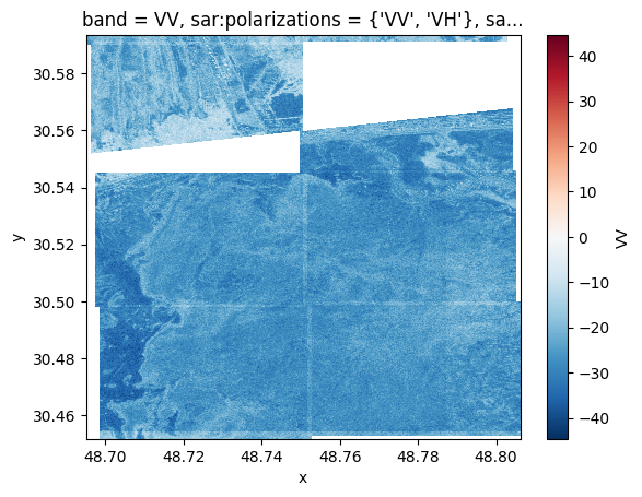
So what does accessing data from the cloud look like? In just a few lines of code, we can instantly pull geospatial metadata describing our ML imagery and labels. With a few more lines we can load image data as an Xarray DataArray and plot it.
import os
from pystac_client import Client

# making a connection to Radiant Earth MLHUB, or another STAC API that requires an API key
MLHUB_API_KEY = os.environ["MLHUB_API_KEY"]
MLHUB_ROOT_URL = "https://api.radiant.earth/mlhub/v1/"
client = Client.open(MLHUB_ROOT_URL, parameters={"key": MLHUB_API_KEY})

# our search requirements
bbox = [46.37225341796875, 25.132194334419058, 50.08224487304688, 30.59343171743452]
time_range = ["2019-04-01", "2019-04-01"]
source_search = client.search(
        collections=["sen12floods_s1_source"], bbox=bbox, datetime=time_range
    )
label_search = client.search(
        collections=["sen12floods_s1_labels"], bbox=bbox, datetime=time_range
    )

# getting the metadata and links to data assets in STAC format
source_items = source_search.get_all_items()
label_items = label_search.get_all_items()

# converting STAC items into an xarray data array, then computing weekly composites
stack = stackstac.stack(source_items, epsg = 4326)
weekly_vv = stack.sel(band="VV").resample(time="1w").mean(dim=("time")).rename("VV")

# making a quick plot
weekly_vv_db_units = np.log10(weekly_vv.isel(time=1))*10
weekly_vv_db_units.plot()Fig 2. The result our data pipeline that queries a STAC API. X is the longitude and y the latitude. The "V V” color bar represents the type of polarity signal for the C-band radar image.
Some upfront work needs to be done to enable this workflow:
-
Use tools like STAC browser to discover existing STAC APIs and guides like this geospatial python lesson for instruction on how to access them.
-
The imagery data needs to be available via a STAC API. If it’s not already available via popular STAC APIs like Microsoft Planetary Computer, NASA CMR STAC, AWS Earth Search, or Radiant Earth MLHub, it means you need to create a STAC catalog with stactools and pystac. Then, you'll need to stand up your own STAC API with existing open source tools like stac-fastapi, pgSTAC, and Franklin and ingest your STAC catalog so it can be searched and queried from your STAC API.
-
Even if the data you need exists in STAC, the specification has evolved over time making some STAC items less compatible with modern geospatial python libraries. The code example above will fail because of missing projection information for STAC items. Discussion of this example and a solution is here.
-
Even if the imagery is associated with STAC metadata, your labels may not be. Labels need to be associated with STAC metadata for imagery using the STAC Label extension.
Data Pipelines
Once you have your dataset in memory, then what? There can be a variety of next steps:
- Data Visualization: Plotting images, evaluating different band combinations
- Data Exploration: Computing zonal statistics, counting how many labels you have across the span of your images to determine validation splits, looking at image histograms to understand how sensor quality matches with your target classes of interest, etc.
- Exporting: you may want to export your dataset to another Analysis-Ready Cloud-Optimized format that supports a particular use case. Maybe you want to take advantage of bleeding edge optimizations that require Zarr or some other array format in the data loading phase. Or maybe you want to distribute the dataset in a particular format for others to consume.
- Data Loading: Converting the in-memory dataset on the CPU to an ML tensor on the GPU (we use Pytorch).
You may in fact want to orchestrate some or all of these processes using the same library or process to reduce code duplication and for a simpler overall ML workflow. We’ve recently explored TorchData and found it to be a pleasant experience for a number of reasons:
| Pro | Con |
|---|---|
| Supports a compositional programming paradigm rather than inheritance, which makes it easier for users to weave their own functionality on top of domain specific libraries (like zen3geo) that are built on top of torchdata. | Some features are yet to be implemented or tested, such as random dataset splitters. There seems to be considerable momentum judging by issue and PR activity, so hopefully TorchData will have a stable release soon. |
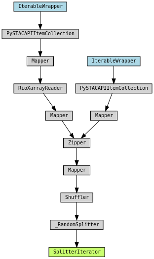
| Can produce handy visuals of data pipelines using graphviz. torchdata.datapipes.utils.to_graph(dp=trn_dp) See Figure 3. | No holistic integration yet with Pytorch-lightning (though we haven’t found this to be a large barrier). |
| Better support for data streams compared to Pytorch’s native Dataloader. |
Fig 3. An example data pipeline that converts a STAC query into tuples of Torch tensors for the image and label pairs. Torchdata allows each step in this datapipe to stream from cloud stores and supports multiprocessing.
Zen3Geo provides geospatial-specific datapipe methods for sourcing data from STAC APIs, loading them as Xarrays, and collating large arrays into smaller samples with xbatcher. It’s proven to be a very accessible and well-documented package that is easy to extend. The compositional nature of Zen3Geo, and it's core dependency TorchData, have several advantages over inheritance based libraries for loading and transforming ML data. Inheritance based data loading libraries are difficult to extend, change, and replace with use-case specific classes. This leads to users rewriting the same code over and over again, rather than writing their use-case specific functions to interoperate with other data pipeline steps. On the other hand, composition can be used to easily chain together and reorder data processing steps that have well defined input and output types. This way, users do not need to subclass library code (like a Torch Dataloader or Pytorch Lightning DataModule) in order to modify, extend, or add data processing steps to a data pipeline. We’ve developed a preference for this style of constructing data pipelines over other geospatial-specific frameworks. This discussion by the maintainer of zen3geo, Wei Ji, outlines a comparison of the predominant GeoML frameworks that largely aligns with our reasons for prioritizing zen3geo.
Data Labeling
GeoML data annotation is complex:
- Data sourcing by the annotation software. The software may only support image uploads, local images on disk, or tile map service URLs (TMS). Supporting this is possibly the largest challenge, as it’s useful to combine datasets when annotating but datasets may not be available in the same standard or format.
- Can the data be easily transformed on the fly? For example, can you compute spectral indices; link displays between one band composite and another to make comparisons? Or make a simple change to the histogram stretch to highlight image variation? GIS tools succeed here, whereas ML annotation tools often don’t support this. See this ENVI doc page for an example of linked displays.
- Support for annotating different detection output types. Common annotation targets include classification, object detection, semantic segmentation, and instance segmentation. Some ML annotation software supports all of these options pretty well. Geospatial annotation tools generally support a subset of these options well but miss important features like model-assisted labeling, semi-automated annotation tools, and a generally fluid UI.
- How the data is exported. Good tools support exporting ML-ready formats or adding labels to existing geospatial metadata standards (STAC). This makes it easier to load annotated image datasets into ML pipelines.
- Human-in-the-loop (HITL) integration. After annotating a dataset, can you train a model and run inferences, then validate those inferences to create additional training data to improve the model score? Few free ML and geospatial annotation tools support this out of the box. Paid services may support this but often miss other key features mentioned above.
With all of these features useful for satellite image annotation, we often need to prioritize some features over others because there isn’t a tool that exists that can do it all. We use OpenStreetMap’s annotation tool, JOSM, for easy sourcing of satellite imagery from TMSs when we need to annotate segments, bounding boxes, or image chip classifications. This requires us to do some upfront work to stand up a TMS, set up derived spectral indices on the fly, or focus on only annotating RGB. Our Data Team has put together a variety of scripts that assist with the input and output of data for ML pipelines: https://developmentseed.org/geokit-doc-seed/
Fig 4. LULC labeling with JOSM. With OSM-seed we can store annotations in a database, allowing our Data Team to divide tasks and conquer large annotation challenges!
When we need to annotate complex segments with 100s of vertices in satellite imagery, we have developed an internal segmentation annotation tool called DS-Annotate (which we will open source in 2023). DS-Annotate has a magic wand feature to quickly annotate similar pixels in segments with an adjustable tolerance and supports custom tile map server URLs.
For on disk, non-geospatial imagery, we prefer CVAT, an open source and free tool that has some support for HITL, an intuitive UI, support for multiple detection types, and is able to export to many ML formats.
Fig 5. Annotating wildlife in Tanzania from aerial imagery for the AI-ASSISTED AERIAL IMAGERY ANALYSIS (AIAIA) TO MAP HUMAN-WILDLIFE PROXIMITY IN TANZANIA project.
Beyond choosing or designing the correct annotation tool, it’s paramount to communicate with the annotation team during the annotation task. There is a growing movement around “Data-centric AI”, which encourages systematic engineering of the systems used to produce quality training data for ML. This approach prioritizes; 1) making sure the annotation task is tightly defined and understood by the annotation team; 2) building or choosing interfaces that annotators can learn and use. In both task and interface design, the collaboration between ML practitioners and annotators is essential. Without it …
“the systemic issues with crowdsourced data annotation continue to torment researchers, product teams, and workers alike. Wages are lost, annotations are tossed.” - “Labeling and Crowdsourcing”
Data Exploration
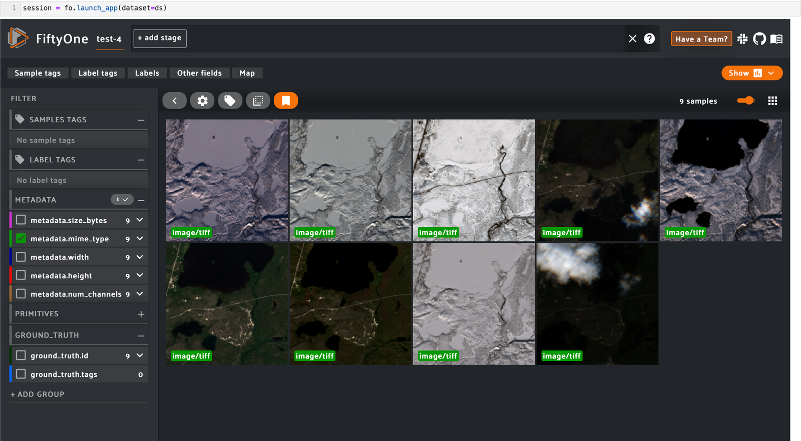
We are currently using FiftyOne, a tool for visualizing annotated image samples, visualizing what a model learns when exposed to data samples, reviewing annotations, and computing evaluation metrics. Check out the core capabilities section to see FiftyOne’s UI and python API for handling data annotations. FiftyOne also has plugins for popular data labeling tools that allow you to integrate this feedback back into your data annotation tool to improve your dataset.
Fig 6. FiftyOne, a tool for visualizing annotated image samples
We primarily use Jupyter notebooks and the python plotting stack to visualize model outputs or embeddings, compute confusion matrices, and inspect performance metrics like precision, recall, and Mean Average Precision (MAP). Notebooks have their benefits in terms of flexibility, but it is cumbersome to write your own evaluation UI for each project. We hope that we can standardize this process by using FiftyOne for dataset and model evaluation and use it to improve how we communicate feedback to our Data Team during the annotation process.
In order to make FiftyOne work for our satellite imagery use case, we need to jump through some extra hoops. FiftyOne runs in the browser, and not all browsers support visualizing local TIFFs. It also doesn’t support all image data types, so bands from Landsat or Sentinel-2 need to be converted to int8. We’ve found the easiest way to support this across multiple browsers is to generate PNG copies of our GeoTIFFs for loading into FiftyOne.
Data Versioning
We are excitedly adopting DVC to version our data, so that we can more easily track past datasets and more quickly reproduce past experiment. DVC creates.dvc files that are tracked in GitHub and DVC can be used to change dataset versions and make checkpoints for new dataset versions. DVC’s solutions for tracking versions of large datasets, (100s of Gbs) will allow us to efficiently store, version, and access data on shared volumes. This will allow us to fully version intermediate datasets within an ML pipeline, where we may be saving remotely fetched datasets from the cloud on an SSD disk or local cloud storage. See more on DVC here.
Data Creation
After sourcing the data and obtaining annotated labels, we need to create an ML-ready dataset that enables our Data Pipeline. We are using Image Labeler and an internal tool to create STAC catalogs for annotated satellite imagery datasets. We are currently working on creating these STACs catalogs with the STAC label extension and the ML AOI extension so that after we ingest them into a STAC API, we can easily load labels and area of interest that matches an ML model's domain. Ultimately, we'd like to unify our work on creating STAC catalogs for ML datasets and incorporate this dataset creation functionality into all of our annotation tools, including JOSM, Image Labeler, and DS-Annotate.
Conclusion
If all those tooling recommendations made you dizzy, you’re not alone. My head’s spinning just thinking about the universe of options for data labeling, pipelines, validation, and versioning. So let’s zoom out a bit.
To recap, our team has recently found a lot of value in standardizing our data pipeline. A lot of the hidden work in ML comes down to good data annotation and lots of data engineering. Simplifying the path from scientific data to in-memory Torch tensors that can be used to train a model is essential for reproducibility and an efficient ML project. Therefore, if you decide to invest time in adopting any of these tools for a GeoML problem, we suggest looking into standardizing your data pipeline by:
1Use STAC
Find an existing STAC API that serves your dataset. If your imagery and labels aren’t in a STAC API, you can use open source tools like stactools to create STAC items that can be ingested into a STAC API.
2Use pystac_client and stackstac
to load STAC Items into Xarray objects for visualization, analysis, and inspection.
3Use TorchData and Zen3Geo
to convert Xarray structures to Torch tensors.
We’re not done yet!
After writing this, we realized that model training, experiment tracking, and serving deserve their own Part 3. Stay tuned for more of us surveying the GeoML tooling landscape for models.
We hope these recommendations for open-source software across the full GeoML stack have been helpful! If you’d like to dig into any of these examples with us or have questions about your GeoML problem, feel free to reach out to ryan(at)developmentseed.com.
What we're doing.
Latest


