Last week in COG Talk 4 we discussed large scale processing using Cloud Optimized GeoTIFF and MosaicJSON. Here is another example on how we can use mosaicJSON and dynamic tiler to create high resolution large scale mosaic.

Divide, Select and Conquer
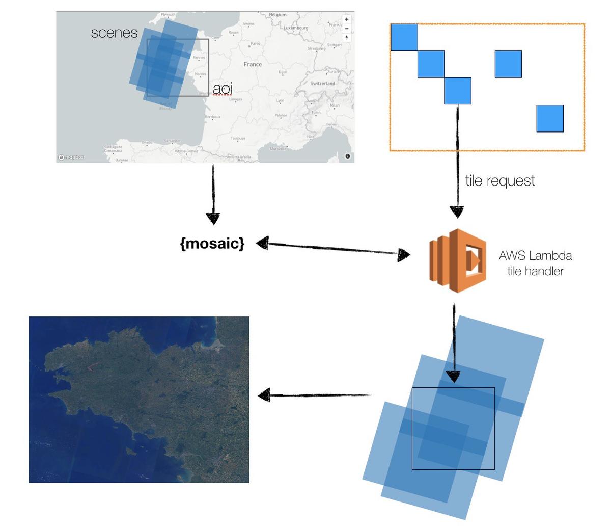
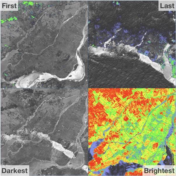
With COG and dynamic tiling you create tiles at the time of request from the raw data. Usually this lets you apply rescaling or color correction to enable a better look for web map display. With mosaicJSON and rio-tiler-mosaic, introduced in COG Talk 2, we extended the idea of dynamic tiling by adding the pixel selection operation. When we have multiple overlapping datasets, you can tell rio-tiler-mosaic which pixel you want to keep or what operation you want to perform on the stack of pixel.
 Pixel selection methods applied on Landsat-8 NDVI values for all 2018 observations over Montreal area.
In this post we want to show how we can use the combination of COGs, dynamic tiler and mosaicJSON to create large scale, good looking and high resolution mosaic of Landsat 8 data.
1. Create mosaicJSON
For this demo, we are using our awspds-mosaic stack. The stack has a mosaic/create endpoint which accepts sat-api queries to create mosaicJSON of Landsat 8 data hosted on AWS PDS.
# Please be kind
# See https://github.com/developmentseed/awspds-mosaic
# to deploy your own
endpoint = "https://landsatlive.live"

# Define AOI here
bounds = [-5.833740234375, 46.15700496290803, -0.9118652343749999, 49.23912083246698]

# Date Filters
start = "2019-01-01T00:00:00Z"
end = "2019-12-31T23:59:59Z"

# SAT-API QUERY
# see http://sat-utils.github.io/sat-api/
query = {
    "bbox": bounds,
    "time": f"{start}/{end}",
    "query": {
        "eo:sun_elevation": {"gt": 0},
        "landsat:tier": {"eq": "T1"},
        "collection": {"eq": "landsat-8-l1"},
        "eo:cloud_cover": {"gte": 0, "lt": 3},  # Cloud Filters
    },
    "sort": [{"field": "eo:cloud_cover", "direction": "asc"}],
}

tilescale = 2  # Each tile will be 512x512px
tilesize = 256 * tilescale

# We post the query to the mosaic endpoint with some optional parameters
results = requests.post(
    f"{endpoint}/mosaic/create",
    json=query,
    params={
        # Landsat covers zoom 7 to 12 but
        # because we don't want to use the mosaic for visualization
        # purpose we don't really care about lower zoom level.
        # We could use zoom 11 but don't want to make the mosaicJSON file too big.
        # Minzoom define the quadkey zoom and thus the number of quadkey list
        # See https://github.com/developmentseed/mosaicjson-spec/tree/master/0.0.2
        "minzoom": 9,
        # We filter the season to have greenest data
        "seasons": "spring,summer",
        # Here we can also pass some tile option to be added to the tile url.
        "tile_format": "tif",  # We use GeoTIFF output from the tiler
        "tile_scale": tilescale,
    },
).json()
In 👆 the above we:
-
define an area of interest (AOI), date range and cloud filter for the SAT API search endoint (Note: it should work the same with any other STAC api)
-
POST the query to the mosaic endpoint with optional parameters (season, tile format…)
The result of the requests is a tileJSON like object.
2. Create list of mercator tiles
We are going to distribute our processes using web mercator tiles at zoom 11 (512x512 px tiles have the same resolution as zoom12 256x256 tiles). For our area of interest, this represents 783 tiles.
# Get Mercator tiles covering the AOI
# For Landsat the maxzoom is 12 (~38m resolution, in Web Mercator projection)
# because we use 512x512 pixel tiles we can
# fetch tiles at zoom 11 instead of 12.
zoom = results["maxzoom"] - (tilescale - 1)

extrema = tile_extrema(bounds, zoom)
tiles = []
for x in range(extrema["x"]["min"], extrema["x"]["max"]):
    for y in range(extrema["y"]["min"], extrema["y"]["max"]):
        tiles.append(mercantile.Tile(z=zoom, x=x, y=y))

random.shuffle(tiles)
3. Create tile URL
In this step we define the creation option for the tiles. The query_params will be added to the tile url obtained in 1.
# Create tile URL
# See https://landsatlive.live/tiles/docs for the list of options you can pass to the tile url
query_params = dict(
    bands="4,3,2", # True Color RGB
    color_ops="gamma RGB 3.5, saturation 1.7, sigmoidal RGB 15 0.35", # Looks nice
    pixel_selection="median",  # See https://github.com/cogeotiff/rio-tiler-mosaic/blob/master/rio_tiler_mosaic/methods/defaults.py#L86
)
tiles_url = results["tiles"][0] + urllib.parse.urlencode(query_params)

def _worker(tile, retry=0):
    """
    Tile Worker.

    Call the tile endpoint for each mercator tile.

    """
    url = tiles_url.format(z=tile.z, x=tile.x, y=tile.y)
    img = requests.get(url)
    if not img.status_code == 200:
        if retry == 3:
            raise Exception("Empty")
        return _worker(tile, retry=retry+1)

    row = (tile.y - extrema["y"]["min"]) * tilesize
    col = (tile.x - extrema["x"]["min"]) * tilesize
    window = Window(col_off=col, row_off=row, width=tilesize, height=tilesize)

return window, img-
**bands="4,3,2"**: We pass the RGB band combination as a coma separated list. Here4,3,2correspond to Landsat 8 band combination for True Color. -
**color_ops="gamma RGB 3.5, saturation 1.7, sigmoidal RGB 15 0.35"**: The Landsat data is stored asUint16data type, in order to obtain a good looking result we apply a rio-color formula. -
**pixel_selection="median"**: This is were the magic happens. The[median](https://github.com/cogeotiff/rio-tiler-mosaic/blob/master/rio_tiler_mosaic/methods/defaults.py#L86) pixel selection option means that for each tile, the dynamic tiler will return the median value for the whole stack of data.
Note: In the _worker function you could likely add an inference step to apply ML on the output tile.
4. Distribute and collect
We now can call the tiler and get the resulting tiles (⚠ it can take up to 1 min). We also use some Rasterio code to merge the tiles into one raster file which we then translate to Cloud Optimized GeoTIFF.
# Define Output COG parameters
width = (extrema["x"]["max"] - extrema["x"]["min"]) * tilesize
height = (extrema["y"]["max"] - extrema["y"]["min"]) * tilesize
w, n = mercantile.xy(
    *mercantile.ul(extrema["x"]["min"], extrema["y"]["min"], zoom)
)
res = _meters_per_pixel(zoom, 0, tilesize=tilesize)

params = dict(
    driver="GTiff",
    dtype="uint8",
    count=3,
    width=width,
    height=height,
    crs="epsg:3857",
    transform=Affine(res, 0, w, 0, -res, n),
    nodata=0,
    tiled=True,
    blockxsize=tilesize,
    blockysize=tilesize,
)
output_profile = cog_profiles.get("deflate")

# Distribute the processes using multithreading
# and then re-assemble the tiles in one COG
with rasterio.Env():
    with MemoryFile() as memfile:
        with memfile.open(**params) as mem:
            with futures.ThreadPoolExecutor(max_workers=50) as executor:
                future_work = [
                    executor.submit(_worker, tile) for tile in tiles
                ]

                for f in tqdm(futures.as_completed(future_work), total=len(future_work)):
                    pass

            for f in _filter_futures(future_work):
                window, img = f
                with rasterio.open(BytesIO(img.content)) as src_dst:
                    mem.write(src_dst.read(indexes=(1,2,3)), window=window)

            cog_translate(
                mem,
                f"Bretagne_medianPixel_2019.tif",
                output_profile,
                config=dict(GDAL_NUM_THREADS="ALL_CPUS", GDAL_TIFF_OVR_BLOCKSIZE="128")
            )
5. The result
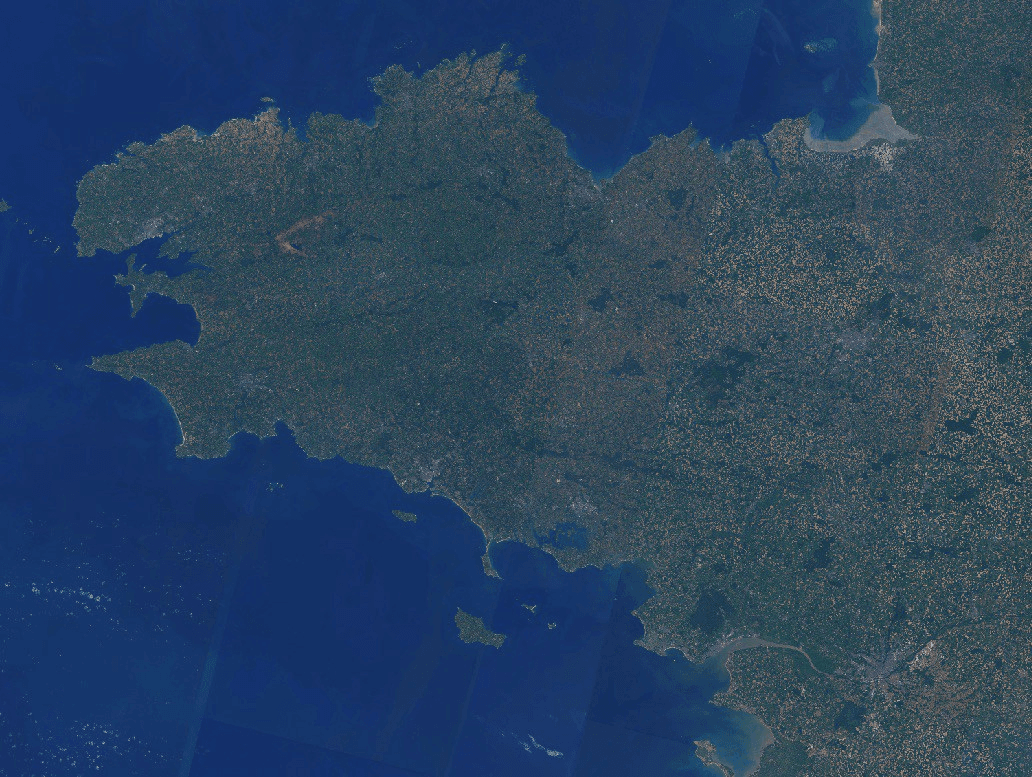
 High Resolution mosaic over Britany using median pixel selection for all 2019’s spring and summer Landsat 8 scenes with less than 5% of cloud.
Doing this over Brittany is great, but can we scale it to a country size area ? 👇
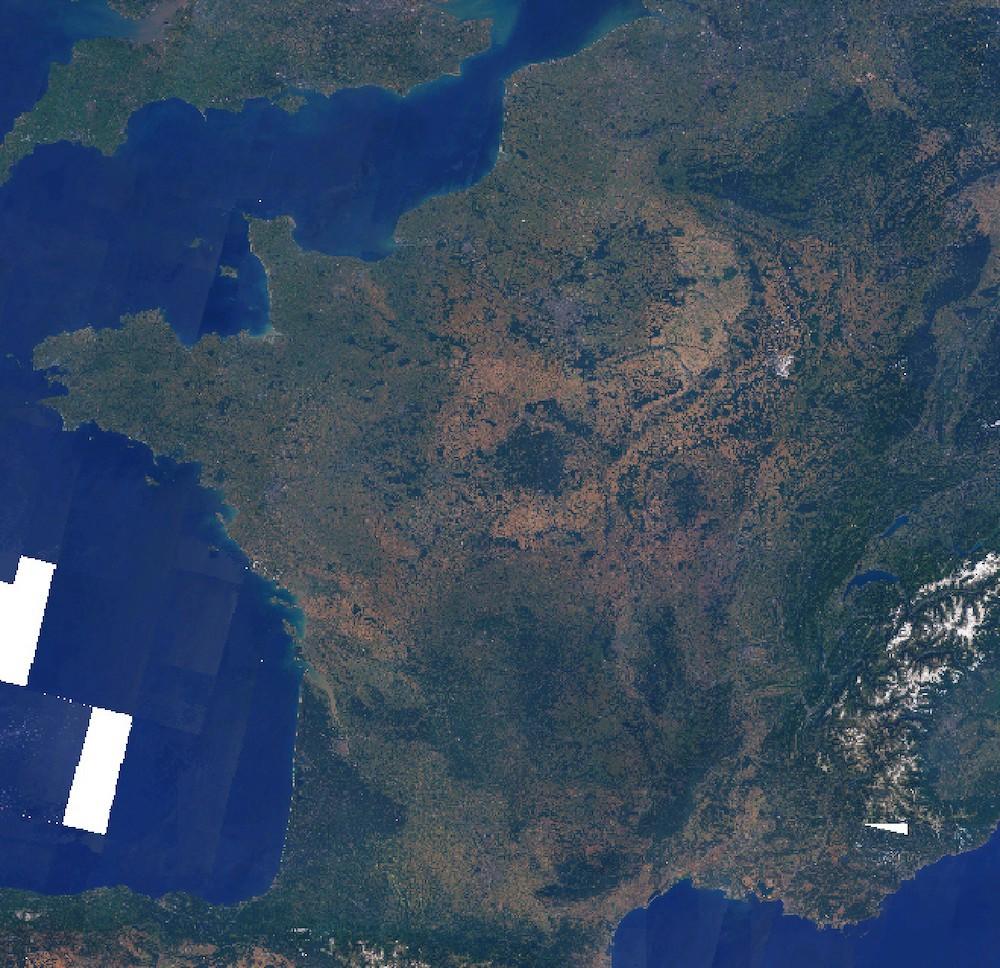
 High Resolution mosaic over France using median pixel selection for all summer Landsat 8 scenes (2013 → 2019) with less than 10% of cloud.
Checkout the high resolution image here.
Doing this over an entire country takes a bit more time, however using AWS Lambda and our cogeo/mosaic-* tools it takes less than 10 minutes 😱. Here are some numbers to put this in context:
-
~7 min for the tiles creation step (it takes almost longer to merge the tiles into one COG)
-
7802 number of Zoom 11 tiles to fetch (== AWS Lambda calls)
-
522 different Landsat 8 scenes (x3 bands)
-
>76 Gb of data fetched (522 x 3 x ~50Mb per file)
-
48128 x 42496 output raster size
The whole notebook can be found here: https://github.com/developmentseed/awspds-mosaic/blob/master/notebooks/LargeScaleMosaic.ipynb
Got Data ?
We’re always looking for interesting problems to tackle using COGs, if you have a raster dataset and want to learn how COG, STAC or mosaicJSON could help, please feel free to ping me on Twitter or LinkedIn ! And if you are interested in joining Development Seed to help us build technology that helps solve global challenges take a look at our open positions!
What we're doing.
Latest
