

Rebuilding a workflow for estimating wildfire CO₂ emissions using cloud-native processing and how openEO changes the way we work with Earth observation data.

During my internship with Development Seed my goal was to explore openEO. Specifically, I explored how it could be used to assess the climate impact (CO₂ emissions) of forest fires in Portugal.
To get started, I worked through the openEO-UDP GitHub repository and, in particular, the Aquatic Plants and Algae notebook. The notebooks in the repo are interactive and provided a solid foundation for developing my own workflow.
The final outcome of my internship is a Jupyter notebook that uses openEO to calculate the difference between two satellite images (dNBR) and apply a machine learning algorithm through a UDF. During my master's thesis I developed a methodology for assessing the climate impact of forest fires using locally processed satellite imagery. During this internship, I operationalized that workflow using openEO, rebuilding it as a cloud-native workflow that performs much of the processing on the server side.
OpenEO
OpenEO is an API for accessing cloud backends to query and process satellite data. This is very useful, because instead of downloading the full image, it allows you to select the relevant data and process it on the server side before downloading. When working locally, you first need to download the entire satellite tile (for Sentinel 2 this covers 110 km x 110 km). This makes it hard to apply the same methodology to multiple images and something like taking a mean of images for one month becomes quickly unfeasible. OpenEO drastically reduces the required local storage and processing power and provides flexibility and efficiency in working with satellite data.
The standard use case is to use openEO to define the spatial, temporal and spectral range you are interested in. You can perform some processing steps such as calculating further indices. Then you can create a job to download the results of the processing to your machine. OpenEO works with lazy n-dimensional data cubes (I had to learn what that was). Lazy means you define the object without loading the data and only load it when you download it. An n-dimensional data cube is a way to represent multi-dimensional data. In this case the dimensions could be time, spatial extent (x,y) and spectral bands.
More information on datacubes.
Detecting Fire Area
For mapping a fire area and understanding exactly the spatial extent of a forest fire the difference in normalized burn ratio (dNBR) can be calculated. Calculating the difference requires the normalized burn ratio for a pre- and a post-fire image.
OpenEO provides a toolbox that is meant to perform processing steps on the satellite-based cubes, such as reducing dimensions or applying a function to the entire cube. The OpenEO toolbox, however, doesn’t explicitly contain a tool for taking a difference between two images within a single cube.
First, I tried to calculate dNBR, by performing the subtraction between two timesteps within a single cube, which was not possible because of indexing issues. The solution I found was to load two separate cubes that each contain one timestep, and only the relevant bands for NBR (4 and 8). They can be subtracted via the merge cubes operation, and the result is the dNBR that indicates how severely each pixel in the bounding box has been burned. At first this did not work, because the merge cubes operation was not available for the EOPF backend. That’s why I switched to the CDSE backend. It supports more functions, including merge cubes.
A takeaway here is that the different backends support different operations and are useful under different circumstances. For example, EOPF processes data much faster, but includes less data (only 2025) and fewer functions.
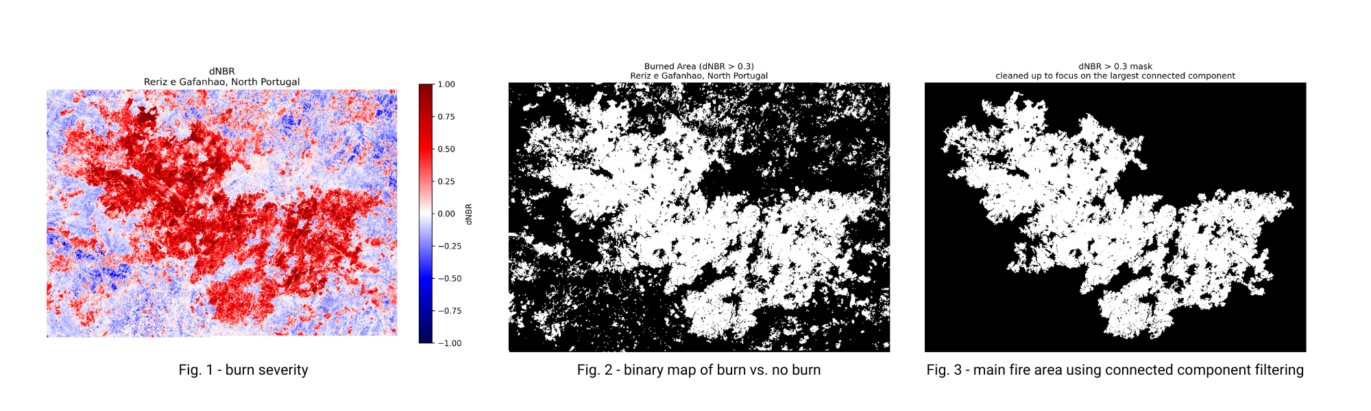
The dNBR gives a continuous indication of burn severity (Fig. 1). To have a binary map of burn vs no burn a threshold of 0.3 is applied (Fig. 2) and connected component filtering is used to delineate the main area of the fire (Fig. 3).
Vegetation Classification
The fire area gives us an indication of the size of the forest fire. However, how much CO₂ was released strongly depends on the type of vegetation that burned. The Portuguese Forest Inventory provides labels of trees in specific points with a relatively low information density (points are 500m apart) (Fig. 4). This doesn’t tell us the distribution of vegetation in the forest yet, but the points can be used as labels for a machine learning algorithm.
A default strategy, and what I also did locally for my master’s thesis, was matching the labels with the corresponding satellite points, training a random forest classifier and predicting a value for each pixel in the forest. Since this project is on openEO, the goal was to outsource as much of this task as possible to the server side.
I loaded a cube with relevant bands and the temporal aggregate (a mean value for each month of the year), which is initialized as a lazy n-dimensional cube. I then loaded the labels as a GeoJson file and applied aggregate spatial to select only the points that have a matching label (500 points), which form the feature space. I downloaded them and now I have the feature space and labels, ready for training a machine learning classifier.
For making a prediction on the entire area, we would need to download the cube containing the entire temporal and spectral range. To avoid this, a UDF is registered. A UDF (user defined function) allows you to write a function that is performed on the server-side. UDFs are programmed to only take cubes as input and give cubes as output, so a previously trained machine learning model cannot be input simply as an object. However, the UDF can take context as input, which allows feeding in a small dictionary (up to 2mb).
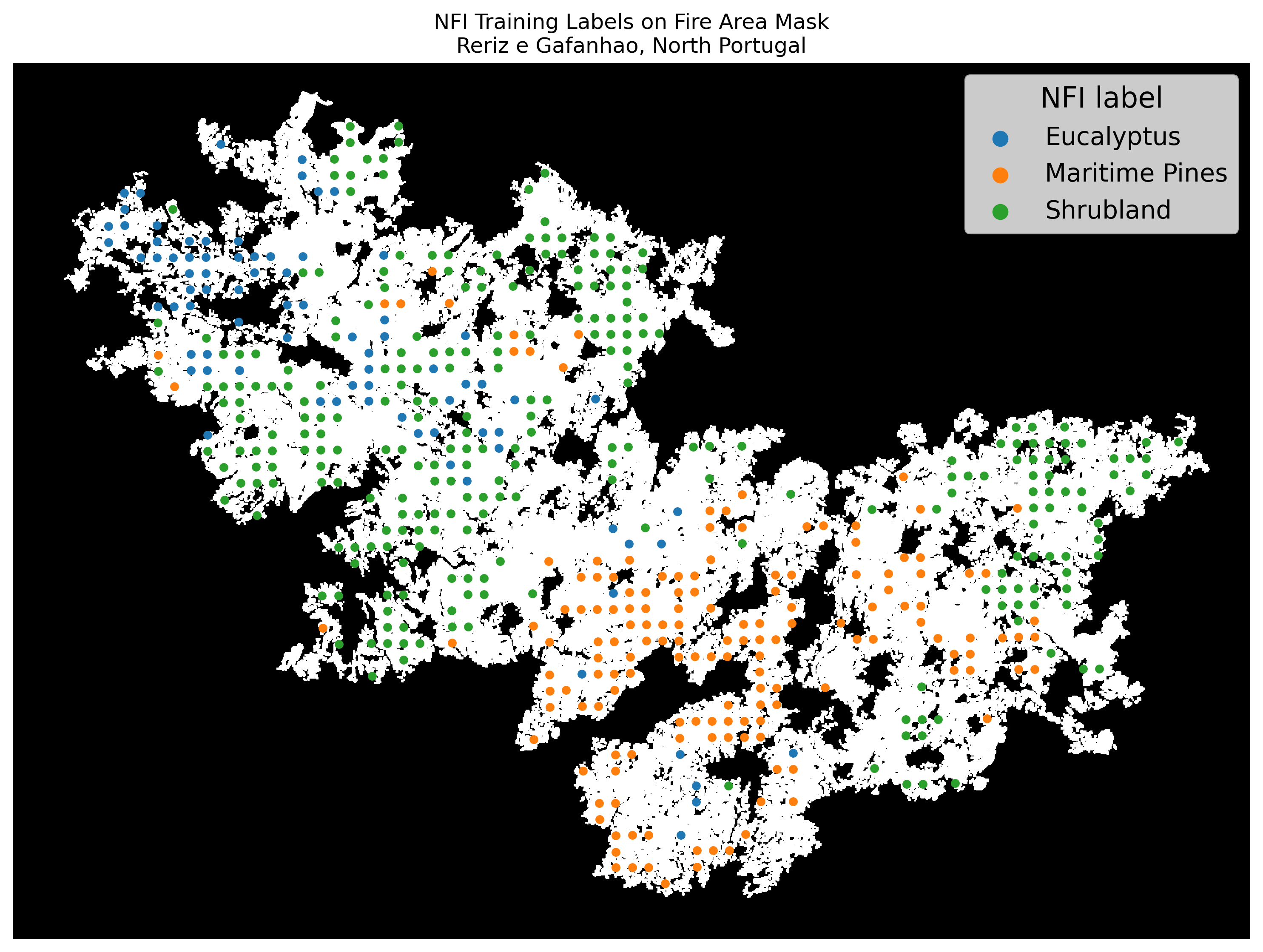
Fig. 4.
The two possible solutions were to either use the context to input the labels and training data and retrain the model within the UDF, or to train the model locally, encode it in bytes and put it into the dictionary and have the UDF parse it back to an object. Both of these options come with some serious disadvantages. Training the model in the UDF means that for every batch the model needs to be retrained (batch means the process is split into sub parts that are run in parallel to make it faster), which leads to redundant calculations. When giving the model as input, the 2mb maximum size of the context is a limiting factor, as more complex models easily grow much larger. In this case limiting the maximum depth of the trees was enough to ensure the model stays within the given size. For efficiency reasons I chose the second option.
With the UDF approach only the few hundred pixels needed for training the algorithm are downloaded for the entire temporal and spectral range. The model is trained locally and then the predictions on the entire fire area are done on the server-side via UDF. That means we only have to download the final predictions of the model for each pixel (on the spatial but not temporal and spectral range) and can visualize them, to understand the distribution of the burned vegetation species (Fig. 5).
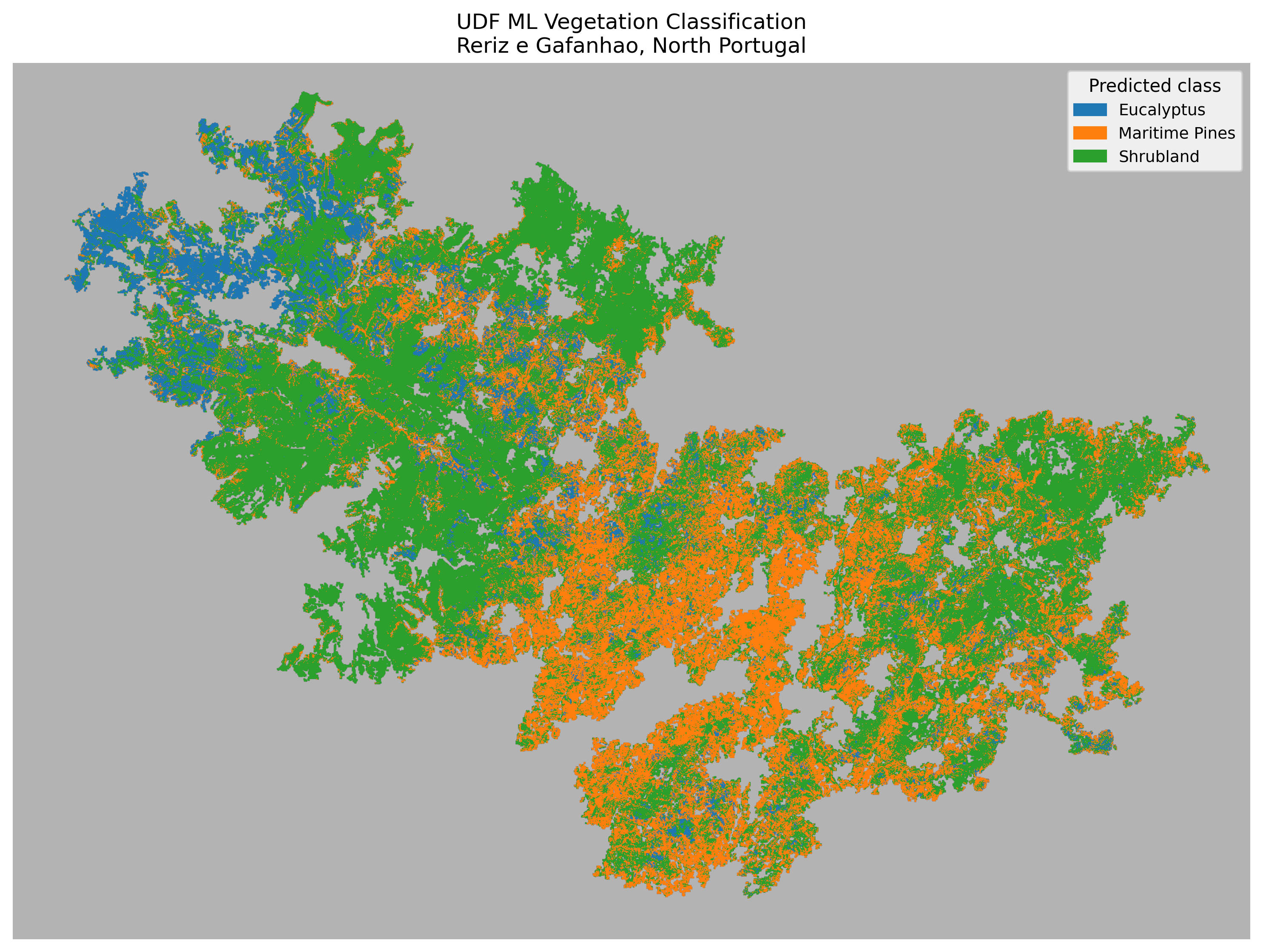
Fig. 5
This work was carried out as a proof of concept and as a result the ML feature engineering was not the focus. The performance of the algorithm could be improved significantly by doing more advanced processing such as using convolutions, including more bands and increasing the area of training data to include more labels.
CO₂ emissions
Calculating how much CO₂ was released during the forest fire can be done through a simple formula with species specific factors. The algorithm predicts what percentage of the forest was covered by which kind of vegetation. Putting in the values (more details in the notebook) gives an estimate of 1.3 million tons of CO₂ released in the forest fire.
This methodology in combination with IPCC values estimates the CO₂ emissions caused by a forest fire. It does so with a resolution of 20m, capturing variation within the burnt area. However, the final CO₂ value was not validated due to an absence of ground-truth. The accuracy of the final prediction depends on the accuracy of the vegetation specific values and the performance of the machine learning algorithm.
This is a use case for making a detailed map of a forest using machine learning.
Overall takeaways of working with openEO
One of the main improvements I have experienced working with openEO is the ease with which you can feature engineer the algorithm. It only takes changing a few lines of code or even just adjusting a parameter to change the bands used for training the machine learning algorithm, or for changing the number of timesteps used, their sampling date and sampling strategy. Working locally this was a huge limitation. Downloading and processing a new satellite image would have taken 1-2 hours, so I was limited to working with 2 individual images rather than with a timeseries. Working locally also required me to work with different programs and then exporting the project. Using openEO also simplified the workflow by allowing me to work within a single environment, rather than moving between tools like SNAP and Python.
All in all, openEO provides a lot of flexibility and generalizability. Applying the same methodology to a different area or increasing the scale becomes easy. However, there are still challenges for significantly increasing the area scale (like mapping all forests in Portugal). Staging context like a large classifier model is still challenging: UDFs don't support inputting a classifier object directly, and the small context size limits how complex a model can be. This forces the developer to integrate the whole workflow, including training, into openEO itself. In this case the study area only contained three vegetation classes. For areas with more vegetation classes more complex models may be needed to achieve good separability between classes. In the future or with different backends it may be supported to feed larger objects into the UDF or to input a larger context, which would allow for larger, more complex models.
What took 1-2 hours locally now takes changing a single parameter.
A counterintuitive thing I observed was that downloading the algorithms prediction on only the area of the fire rather than the larger bounding box is much less efficient, even though the fire area contains significantly fewer points. This is because the points in the fire mask have to be represented as vectors (GeoJson) rather than a continuous raster (GeoTiff), which is a less efficient way of storing the data. As a result, downloading as a GeoJson only supported up to 10,000 points, whereas a GeoTiff handled 2 million pixels without an issue.
Outlook
As shown in this use case, classifying vegetation species that burned during a forest fire has practical applications. Combined with species-specific emission factors, it provides a way to estimate CO₂ emissions at a 20-meter resolution, capturing variation within the burned area.
With further validation and development, workflows like this could help inform larger-scale CO₂ estimation efforts by providing more detailed information about burned vegetation.
More broadly, this project explored how openEO can be used to build a cloud-native workflow for assessing the CO₂ emissions of a forest fire. It also explored how machine learning can be applied through a UDF and highlighted some of the current limitations of that approach.
One of the biggest takeaways from this internship was realizing that openEO can support much more than data access and preprocessing. At the same time, working through the limitations of today's server-side machine learning workflows gave me a better understanding of where the technology is today and where it has the potential to evolve in the future.
You can explore the notebook I created and try it for yourself. To continue the conversation you can find me on LinkedIn.
What we're doing.
Latest