This guide is for machine learning practitioners looking to apply Keras models at scale. I’ll cover a concrete problem we faced and then provide a code walkthrough of our solution.

Finding electricity infrastructure at scale

Access to electricity is a major issue in parts of the developing world. So much so that the United Nations specifically allotted one of its 15 Sustainable Development Goals (specifically, #7) to “ensuring access to affordable, reliable, and modern energy for all.” Many organizations are working hard to improve energy access around the world, but it’s often difficult to find maps of the existing electric grid. Without infrastructure maps, these groups are essentially blind as to where to invest resources for infrastructure improvement or opt for off-grid solutions (e.g., solar and wind power).

In a previous project, we’ve shown that artificial intelligence can speed up the generation of these electricity infrastructure maps. High-voltage (HV) transmission towers are stereotypical structures tens of meters tall making them relatively easy for humans (and machines) to find in satellite images. With a few thousand training samples, we trained an ML model to flag satellite images containing these towers. We could then use this model to quickly generate an initial map of a network’s backbone by highlighting likely HV tower locations. Eventually, this ML-derived information helped our mappers generate complete electric grid maps about 30x faster than a purely manual mapping approach. However, achieving that 30x gain was a major hurdle because it required applying our trained model to country-sized imagery datasets.

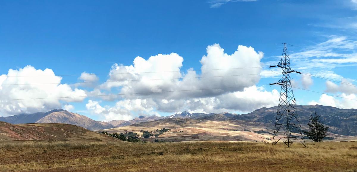
High voltage towers in Peru near the Andes. Photo credit: Laura Gillen

Processing 120 million images

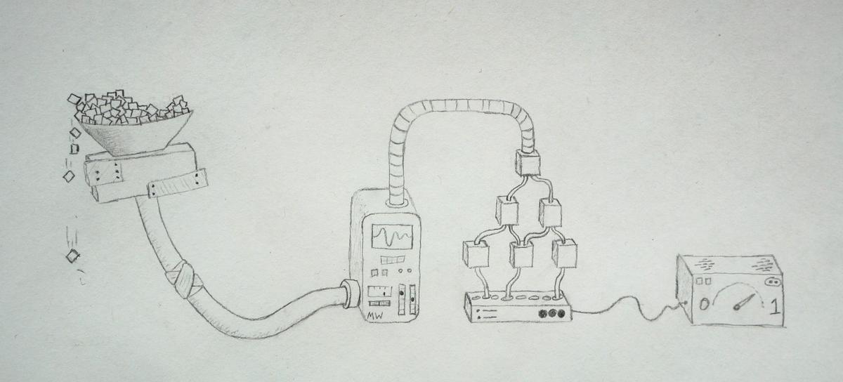
The pain began to crescendo when running inference (or prediction) on the 120,000,000 satellite images tiling our three target countries: Nigeria, Pakistan, and Zambia. We manually managed 5 GPU instances on Amazon’s EC2 with each instance processing a new batch of images every 5–6 hours. Shortly after each batch was complete, we needed to manually prepare a new image batch and restart the cycle. Our timeline was tight and required keeping these machines running at full bore for almost 2 weeks straight. It was an impractical, less-than-graceful pipeline that sometimes felt as if it was held together with the digital equivalent of spit and glue.

The rest of this blog post covers how we grew out of that struggle. After a deep retrospective, strategy pivot, and tool belt upgrade, we’re now able to run ML inference on tens of millions of tiles per hour with almost no manual monitoring. A significant chunk of this transition relied on a tool called TensorFlow Serving.

Before TF Serving

Introduction to TF Serving

TF Serving helps package up a Keras (or TensorFlow) model as a Docker image. This has many benefits, but three are very practical:

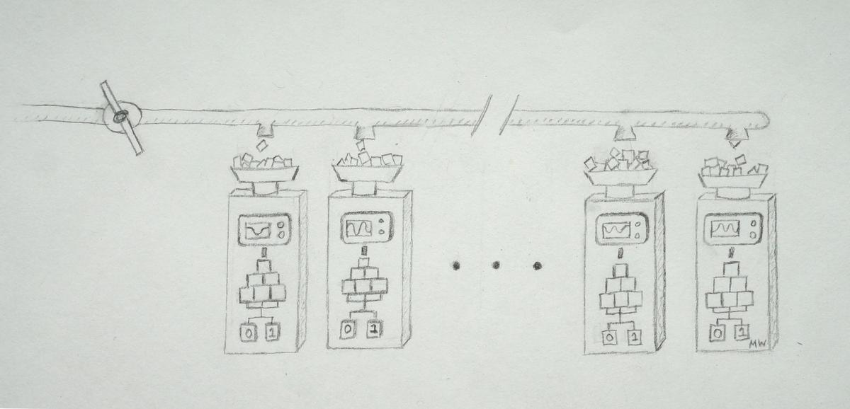
1. Parallelized scaling: Once you’ve built your Docker image, you can stamp out multiple clones of your model to trivially scale up inference speeds. For satellite imagery, this allows us to go from city-wide to country-wide scale very quickly.

2. Sharing: Docker has a service to host images on DockerHub. Once you’ve pushed your TF Serving image to DockerHub, any computer that is capable of running Docker (i.e., almost any laptop, desktop, or cloud server) can also run your ML model.

3. Real-world deployment: TF Serving images act as a small server that exposes a RESTful API. This means you can send inference requests and receive inference results using a standardized protocol that works over the internet.

After TF Serving

Code walkthrough: generate TF Serving image from Keras model

Let’s get into the code. We’ll break down the tutorial into 3 parts:

1. Export a model that’s ready for containerized deployment

2. Package the exported model into a TF Serving Docker image

3. Send inference requests to our deployed model

1. Exporting an inference-ready model

First, we need to make sure proper preprocessing is applied, which is especially relevant for computer vision models. The Xception model, for example, requires conversion of uint8 values [0, 255] to a float on the interval [-1, 1]. In model training, this often happens outside of the model itself (e.g. in an image augmentation step. If that’s the case, we need to add that preprocessing to our inference computation graph. Make sure to update the function below if you need to scale your pixel values differently. More details on the serving_input_receiver_fn are on TF’s Save and Restore guide.

import os
import os.path as op
import tensorflow as tf

HEIGHT, WIDTH, CHANNELS = 256, 256, 3


def serving_input_receiver_fn():
    """Convert string encoded images (like base64 strings) into preprocessed tensors"""

    def decode_and_resize(image_str_tensor):
        """Decodes a single image string, preprocesses/resizes it, and returns a reshaped uint8 tensor."""
        image = tf.image.decode_image(image_str_tensor, channels=CHANNELS,
                                      dtype=tf.uint8)
        image = tf.reshape(image, [HEIGHT, WIDTH, CHANNELS])

        return image

    # Run preprocessing function on all images in batch
    input_ph = tf.placeholder(tf.string, shape=[None], name='image_binary')
    images_tensor = tf.map_fn(
        decode_and_resize, input_ph, back_prop=False, dtype=tf.uint8)

    # Cast to float32
    images_tensor = tf.cast(images_tensor, dtype=tf.float32)
    #  Run Xception-specific preprocessing to scale images from [0, 255] to [-1, 1]
    images_tensor = tf.subtract(tf.divide(images_tensor, 127.5), 1)

    return tf.estimator.export.ServingInputReceiver(
        {'input_1': images_tensor},  # The key here needs match the name of your model's first layer
        {'image_bytes': input_ph})   # You can specify the key here, but this is a good default

With the image preprocessing function written, we’re going to export our Keras model now. We’ll convert the model to a tf.estimator object, which is a high-level format that will make it easy to export the model as a tf.saved_model (explained in detail here).

# Define a place to save your compiled model
export_dir = '/path/to/my_exported_models/001'

# Define a path to your trained keras model and load it in as a `tf.keras.models.Model`
# If you just trained your model, you may already have it in memory and can skip the below 2 lines
model_save_fpath = '/path/to/my_model.h5'
keras_model = tf.keras.models.load_model(model_save_fpath)

# Create an Estimator object
estimator_save_dir = '/path/to/save/estimator'
estimator = tf.keras.estimator.model_to_estimator(keras_model=keras_model,
                                                  model_dir=estimator_save_dir)

Try running the line below to export our tf.saved_model object. Unfortunately, TF might not quite set up the directory structure correctly. If running the next line causes TF to throw errors about a missing checkpoint file, copy the .checkpoint file from the .../estimator/keras directory up one level to the .../estimator directory and then rerun.

# The below function will be renamed to `estimator.export_saved_model` in TF 2.0
estimator.export_savedmodel(export_dir, serving_input_receiver_fn=serving_input_receiver_fn)

Depending on your verbosity settings, TensorFlow may print out some relevant info at this point. It will tell you where the Keras model was loaded from, information about the TF SignatureDef (here, we’re interested in Predictand the serving_defaultkey), and the location of the tf.saved_model object that now includes your preprocessing function.

TF will save your inference-read model to a time-stamped directory under export_dir. You should see your saved_model.pband its weight variables in a directory like /path/to/my_exported_models/001/1548701206.

2. Packaging your model in TF Serving

Now, we’ll build a TF Serving Docker image. This will make it easy to pull and deploy our ML model to any computer connected to the internet. The code below mostly borrows from TF official Docker example here.

Usually, I copy the contents of my exported model up one directory from something like .../my_exported_models/001/1548701206/ to .../my_exported_models/001/ thereby removing the timestamp directory. I recommend doing this as it’ll also allow you to easily call different version of the same model from that one Docker container (if you add a model versions 002, 003, etc.).

Run the following from your command line:

######################################
# Pseudocode for creating Docker image

# Get the Docker TF Serving image we'll use as a foundation to build our custom image
docker pull tensorflow/serving

# Start up this TF Docker image as a container named `serving_base`
docker run -d --name serving_base tensorflow/serving

# Copy the Estimator from our local folder to the Docker container
# You can rename `my_model` to best reflect your model's name. It's what will be used in the REST API call
docker cp /path/to/my_exported_models serving_base:/models/<my_model>

# Commit the new Docker container and kill the serving base
docker commit --change "ENV MODEL_NAME <my_model>" serving_base <org_name>/<image_name>:<version_tag>
docker kill serving_base

###################################
# Same example with filled in data:

docker pull tensorflow/serving
docker run -d --name serving_base tensorflow/serving
docker cp models_hvgrid_export serving_base:/models/hv_grid
docker commit --change "ENV MODEL_NAME hv_grid" serving_base developmentseed/hv_grid:v1
docker kill serving_base
docker run -p 8501:8501 -t developmentseed/hv_grid:v1

You can create also a GPU enabled Docker image by instead pulling tensorflow/serving-gpu and repeating the above code. In that case, tag your GPU model with something like v1-gpu. As in the code above, run the image locally on port 8501 with something like: docker run -p 8501:8501 -t developmentseed/hv_grid:v1. Check that the model is running and get its metadata by visiting something similar to [http://localhost:8501/v1/models/hv_grid/metadata](http://localhost:8501/v1/models/hv_grid/metadata.)

You can also push your Docker image to Docker Hub for easy sharing: docker push <my_org>/<image_name>:<image_tag>

3. Sending inference requests to a running model

Finally, we’re ready to send images to our running Docker container server for inference.

The main wrinkle here is to Base64 encode our data, which is a way of encoding binary data as a string. If you naively tried to send preprocessed images (e.g., as float32 image data), TF will let you. You’ll naively transmit your image data as a string (digits, decimals, and all) and then force your inference server to convert everything to a tensor. However, this is terribly inefficient.

By instead keeping images as data type uint8, base64 encoding the image data, and doing preprocessing with our serving_input_reciever_fn on the server side, I found empirically that the prediction payload size was about 45x smaller for standard 256x256x3 pixel satellite images. This is especially crucial for batch processing of large imagery large sets — smaller payloads mean (1) faster network transmission to your container’s RAM and (2) faster memory transfer from RAM onto our GPU card for processing. It’s vital to keep these transfer times short because it means you’ll keep your GPU utilization (and inference throughput) high. For more background info on sending/receiving data, see TF’s RESTful API explainer page.

Note: you can change your server_endpoint below in when you want to run the Docker container on the cloud — just make sure the appropriate port (8501 by default) is exposed and substitute your instance’s IP address for localhost.

import json
import base64
import requests

# Modify the name of your model (`hv_grid` here) to match what you used in Section 2
server_endpoint = 'http://localhost:8501/v1/models/hv_grid:predict'
img_fpaths = ['path/to/my_image_1.png', 'path/to/my_image_2.png']

# Load and Base64 encode images
data_samples = []
for img_fpath in img_fpaths:
    with open(img_fpath, 'rb') as image_file:
        b64_image = base64.b64encode(image_file.read())
        data_samples.append({'image_bytes': {'b64': b64_image.decode('utf-8')}})

# Create payload request 
payload = json.dumps({"instances": data_samples})

The payload json must abide by a strict structure. If we were to print it out, it should be structured something like this (likely without the newlines):

{
  "instances": [
    {
      "image_bytes": {"b64": "iVBO...Oxs6"}
    },
    {
      "image_bytes": {"b64": "0KGg...Pyg8"}
    },
    {
      "image_bytes": {"b64": "AABr...EKA0"}
    }
  ]
}

Now let’s send the encoded image payload for inference:

# Send prediction request
r = requests.post(server_endpoint, data=payload)
print(json.loads(r.content)['predictions'])

If everything works, you should get back some json content containing your model’s inference output! With a fairly standard XCeption architecture, we were able to process about 1,600,000 satellite images tiles per hour on two p3.2xlarge AWS instances (running V100 GPUs). Good luck and make sure to poke around for newer solutions as the TF Serving codebase (and ML inference more generally) is evolving quickly.

Other tricky bits

• TensorFlow relies on aSignatureDef to specify how you will provide input data. We’ll usually use the Predict signature definition (indicated by the :predict suffix on our POST request in Section 3). There are a couple different ways to send inference requests though, and you can read more details and about the Classify and Regress SignatureDefs on TF’s SignatureDef page.

• TensorFlow is picky about many of the keys used when moving data throughout this pipeline. You need to make sure that:

1. The tensor name in your serving_input_receiver_fn's return statement matches your Keras model’s input layer name. (Here, this was input_1 as in Section 1).
2. The tensor name in your serving_input_receiver_fn's return statement matches the key used in your json key for each sample to be predicted. (Here, this was image_bytes as in Sections 1 and 3).
3. You keep the b64 key for base64 data. This tells TensorFlow to decode the string data back into bytes.
4. You keep the instances key in our json payload. This lets TF know that there is a batch of data coming. See TF’s REST API page for more information.

• REST vs gRPC. The RESTful API is relatively new for TF. Google’s Remote Procedure Call (gRPC) is another protocol for interfacing with TF serving models that is supposedly faster but more complicated. Personally, I wasn’t able to get it up and running, but there is at least one comparison out there if you want to test it out.