Using unsupervised clustering to create training data for machine learning models

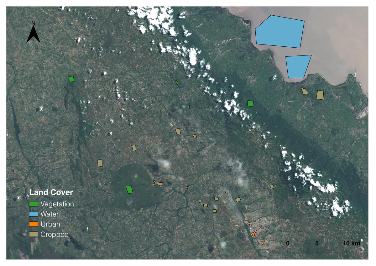Sentinel-2 image near Sumbawanga, Rukwa, Tanzania. Polygons were created manually in GQIS and used to generate “ground-truth” data for clustering and classification.

Gaining a better understanding of where crops are being produced and how they are performing will be an important component of connecting smallholder farmers in developing countries to increasingly globalized value chains. Development Seed is exploring ways to more accurately and efficiently predict where specific crops are being grown using newly available Satellite imagery.

Before providing an update on our progress, a brief recap of the project’s approach: We are exploring an alternative method for generating training data for machine learning models using Sentinel-2 satellite data. Rather than relying on large quantities of geo-referenced crop locations taken from actual fields, we’re testing the feasibility of labeling groups of pixels based on temporal trends of their NDVI values. The logic is that NDVI curves of pixels representing the same crop type will have similar characteristics and can therefore be grouped together and labeled. The first post in this series provides a more in-depth discussion of the rational and methodology for this approach.

In Part 1 of this series, we introduced some of the problems associated with predicting the locations of specific crops in challenging geographies. Leveraging Sentinel-2 data on the Earth on AWS platform, we are exploring some possible solutions. Briefly, the problems can be grouped into several categories:

1. a lack of “ground-truth” data of known locations where specific crops are being grown

2. small and irregular plot sizes typical of developing countries (limiting the effectiveness of low- and medium-resolution satellite imagery for these regions)

3. the diversity of crops and cropping systems practiced in relatively small areas.

In Part 2 of this series, we’ll provide an update on the progress we’ve made thus far. Specifically, we’ll take a look at the results of the clustering phase of the problem. This step refers to the process used to group and label the NDVI curves of individual pixels corresponding to cropped area from a Sentinel-2 scene.

Extracting NDVI cuves

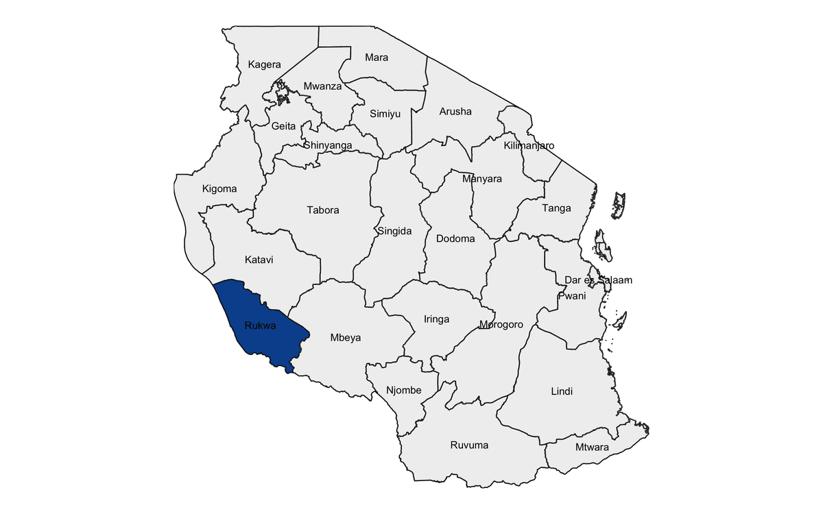
As discussed in the first post of this series, we selected the Rukwa Region of southern Tanzania as an area of interest (AOI) for this project. Rukwa is a major maize producing region and has a single growing season corresponding to a unimodal rainy season.

NDVI is a vegetation index that can be created for a given satellite image using the values in the red and near-infrared (NIR) bands of the scene. NDVI is useful for classifying land cover because different categories of vegetation and other land cover types tend to exhibit specific and recognizable patterns in NDVI. For example, water will typically have a negative value, while bare soils tend to have very low but slightly positive values. Land planted to a crop will generally have NDVI values typical of bare soil at the start of a season, and will increase as the canopy fills in. The shape of a crop’s NDVI curve therefore represents unique characteristics of that crop such as the planting and harvest date, and the canopy structure at peak growth.

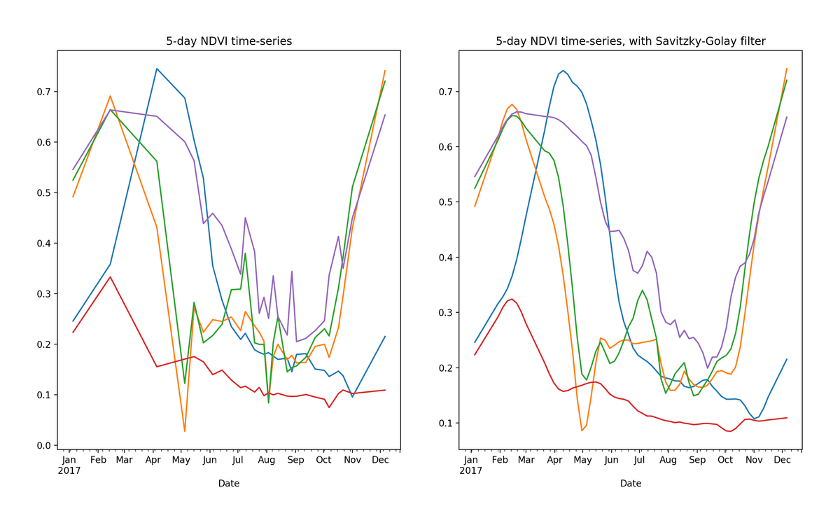Raw (left) and smoothed (right) 5-day NDVI time-series extracted from 5 random pixels in cropped area of Rukwa Region, Tanzania.

As an example, the blue curve in the image above represents a crop planted some time in November, reaching peak growth in May, reaching a maximum NDVI value of around 0.75. Based on the cropping calendar for this region and the overall shape of the curve, there is a good chance that this pixel represents maize. For a visual check, it’s possible to compare publicly available NDVI curves from Malawi — a neighboring country in the same agro-ecological zone.

To build the NDVI curves, we used sat-search (part of the sat-utils toolkit built by Development Seed) to find all Sentinel-2 scenes for the 2017 growing season that intersected with the polygons shown in the image at the top of this post. Sat-search is run in the command line and can be used to search the Sentinel-2 catalogue as follows:

# Install the latest version of sat-search
pip install satsearch=='1.0.0b10'

After installation, execute a search:

sat-search search \
    -p c:id=sentinel-2-l1c \
    -p eo:platform=Sentinel-2A \
    --intersects aoi.geojson \
    --datetime 2016-11-01/2017-12-31 \
    --eo:cloud_cover 0/15 \
    --save scenes.json

The above query saves the metadata associated with all Sentinel-2A scenes with <15% cloud cover between November 1, 2016 and December 31, 2017 in a file named “scenes.json.” The search is limited to those scenes that intersect with the AOI polygon “aoi.geojson.”

The following command downloads the specified bands (assets) from their S3 bucket locations to a directory structure organized by date.

sat-search load scenes.json --download B02 B03 B04 B08

The above command downloads the red (B04), blue (B02), green (B03), and NIR (B08) bands form the Sentinel-2A scenes specified in “scenes.json.” For more information on the work we’re doing to improve how public satellite datasets are catalogued and queried, please read this post.

After converting the images to GeoTiff format using GDAL command line tools, we created NDVI scenes for each date using the “algorithms” functionality from the GIPPY library. For each pixel in the land cover classes shown at the top of the page, we extracted a time-series of NDVI values by first rasterizing the shapefile containing the land cover polygons, and then creating a “mask” to keep only those NDVI values that intersect with the land cover polygons for each class.

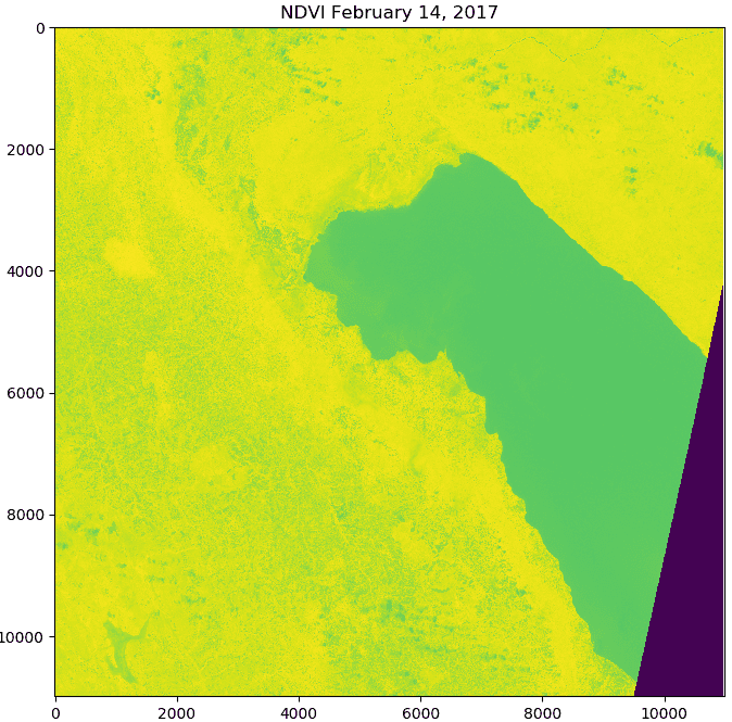
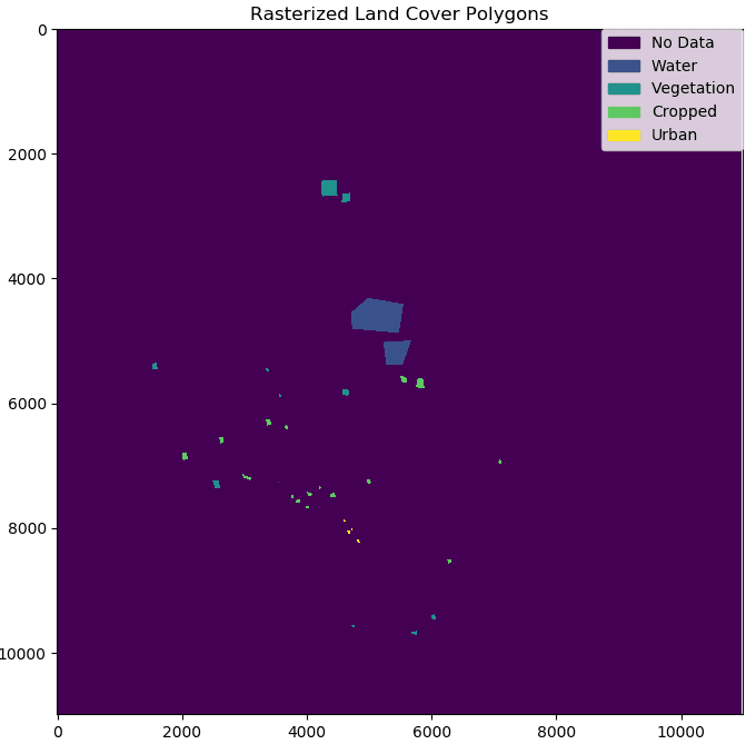An NDVI scene created from Sentinel-2 bands (left), and rasterized land cover polygons (right). For each land cover class show in the image on the right, NDVI values were extracted for all pixels for each NDVI scene in the time-series.

Clustering NDVI curves for cropped area

The good news is that some of the land cover classes we are hoping to classify already have labels. For our purposes, the “vegetation”, “water”, and “urban” pixels labeled by eye using the Sentinel-2 scene at the top of the page do not need to be further separated into sub-groups. The clustering portion of this project therefor relates only to the “cropped” areas. We would like to find natural groups of these pixels, based on how their NDVI values change throughout the growing season, hopefully corresponding to individual crops.

The Sentinel-2 constellation has a 5-day revisit rate. After filtering to keep only those scenes in the 2017 growing season that had a cloud cover of under 15%, we were left with 28 scenes total. To create a more complete NDVI time-series for each of the pixels, we used simple linear interpolation to fill in missing values. The resulting curves had values at 5-day intervals, matching the Sentinel-2 revisit rate.

We used the functionality from the tslearn library to test different clustering techniques specific to time-series. To find a “best” model, we tested different combinations of model parameters, including distance metrics (dynamic time warping vs. soft dynamic time warping), clustering algorithms (K-means vs. global alignment kernel K-means), and the number of clusters. We used the average silhouette score from the resulting clusters as a guide for selecting our final datasets, although ultimately there is a great deal of subjectivity in this process.

We settled on the use of dynamic time warping as a distance metric for comparing the NDVI curves for cropped area pixels, and k-means for a clustering algorithm. We clustered 10,000 pixels from the cropped area using 4, 5 and 6 clusters. The results are shown below:

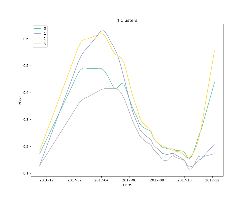
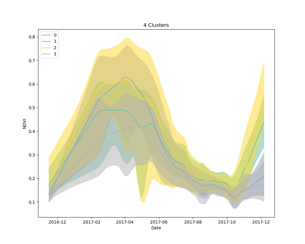
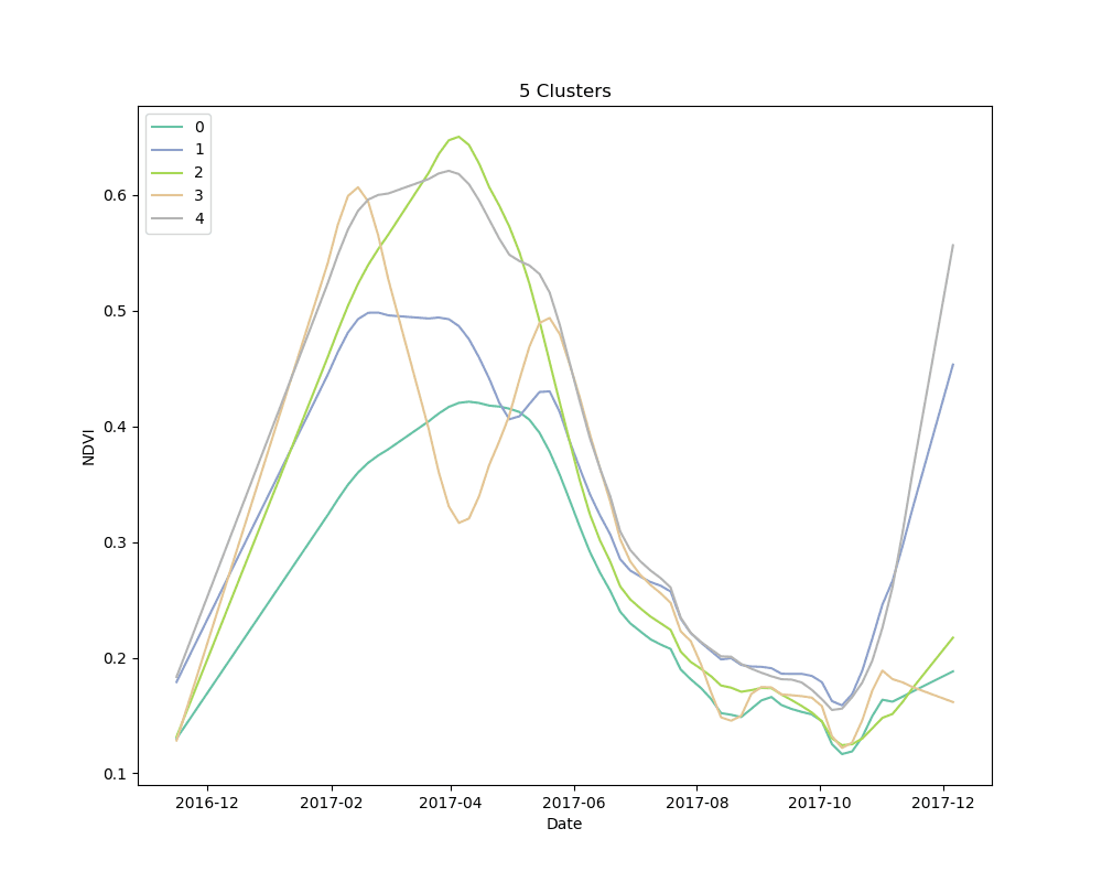
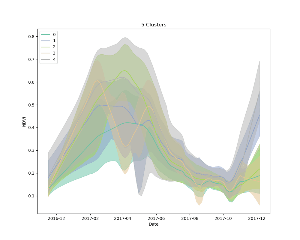
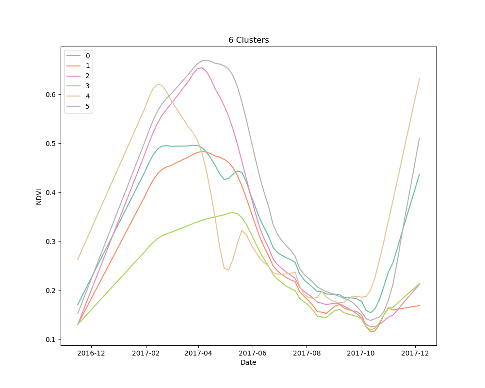
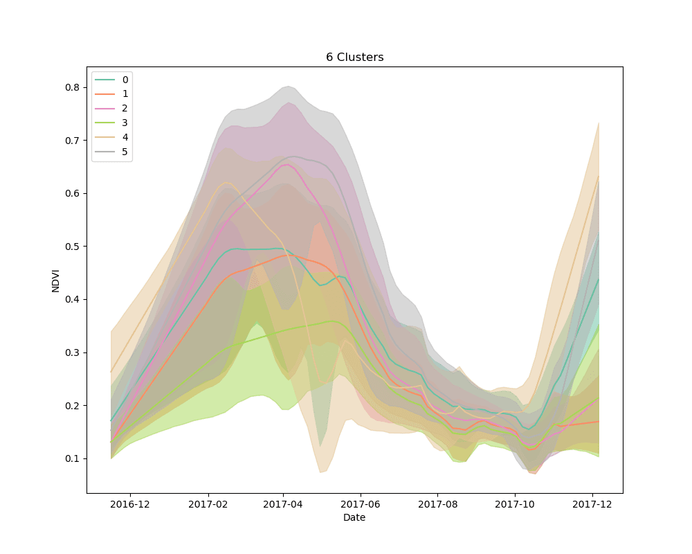Mean NDVI of each cluster for all dates in the time-series. Shaded areas show the 10th and 90th percentile NDVI values from each cluster for all dates in the time-series.

As can be seen from the plots above, it appears that some clusters are relatively consistent despite the total number of clusters in the model. This is encouraging, as it could be an indication that these groups correspond to distinct crop types.

Lessons learned

Unsupervised learning, such as the clustering technique discussed here, is a bit of a dark art. There is no perfect metric for determining the “best” clustering algorithm, and it is impossible to know with certainty what the resulting groups represent in the real world. We knew this going in, but it is useful to highlight the process for selecting a final set of models. We used silhouette scores as a loose guide to settle on a set of hyperparameters for the clustering algorithm, but ultimately decided to test the classification models with more clusters than the silhouette score suggested was “best,” based on a a visual examination of the mean cluster curves (shown above).

Clustering, depending on the distance metric used, is also very computationally intensive. Clustering 10,000 time-series with 78 values each (after interpolation) took approximately 8 hours on an M4 Large AWS EC2 instance. Unfortunately, because the distance from each time series to all other time series must be computed, the options for parallelizing code are limited.

Next steps

Ultimately, we are interested to see how well we can predict the location of individual crop types using satellite images captured during the current growing season. This means building machine learning models for classifying crop types using labeled training data. As a first step, we will see how effectively we can predict to the clusters themselves, without worrying about labeling them as specific crop types and using only the first few images from the growing season. This should give us an indication of the potential usefulness of the cluster labels, and provide guidance on how best to proceed with the labeling portion.

We will provide a final post detailing the classification portion of this project, in which we label the clustered cropped area pixels and predict the spatial extent of maize in the 2017 growing season. We can then compare this value with the reported maize area from the Tanzania agricultural survey to get a rough sense of the accuracy of the crop labels. Stay tuned.