


The Jupyter ecosystem is growing to meet fast, large scale data science, collaboration and publication.

Since 2011, Project Jupyter has radically changed scientific computing by introducing browser-based interactive environments that combine code, visualizations, maps, and other elements.
Jupyter Notebooks and hosted services like Google Colab have become the de facto standard for modern data science workflows, including geospatial data analysis. Operating entirely within web browsers, notebooks enhance research shareability, readability, and collaboration, especially when integrated with version control platforms like GitHub.
This approach accelerates the iterative process of prototyping analyses and creating visualizations. This is particularly valuable with today's unprecedented data volumes and complex methodologies. Powered by the JupyterHub infrastructure, these notebooks support an array of scientific programming languages, including Python, R, and Julia, enabling the data science community to code, visualize, share, and publish their work efficiently. As a result, over the last ten years, Jupyter has significantly streamlined scientific analysis and publication workflows across many domains.
Jupyter is a window that enables fast geospatial research directly in the browser.
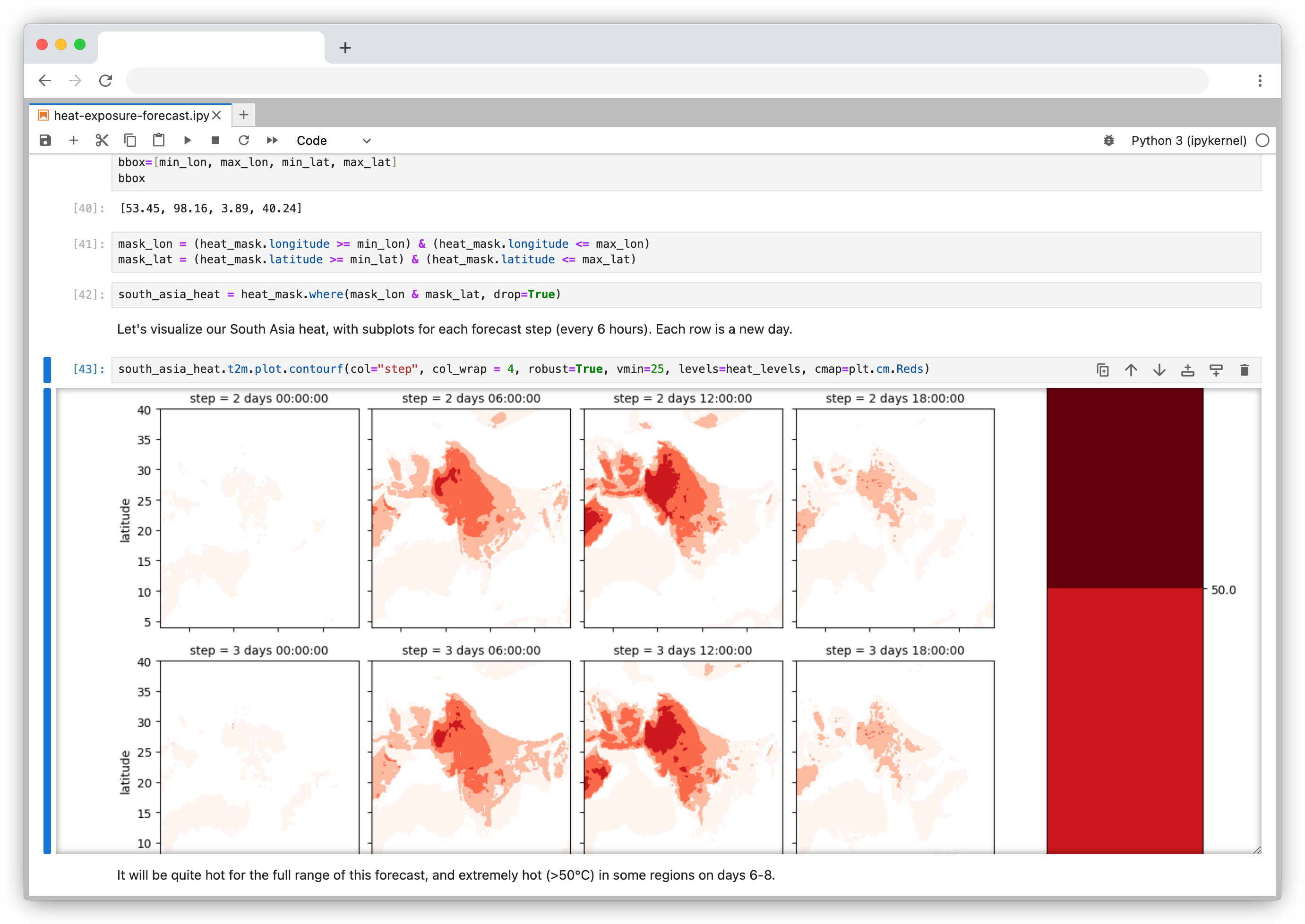
Heat forecast analysis in Jupyter notebook using ECMWF data
Geospatial in the browser
Geospatial analysis has evolved significantly over time. Traditionally, scientists relied on desktop Geographic Information System (GIS) software like QGIS and ArcGIS, which focused on map creation. These tools typically began with datasets and culminated in static, publication-ready maps.
However, the Jupyter ecosystem has transformed this workflow, shifting more analysis to web-based environments. This transition has addressed some inherent challenges in geospatial analysis, particularly regarding reproducibility and collaboration. Jupyter technology makes it easy for notebooks to be run locally or in the cloud, allowing scientists not to be limited by what their computers can do. This flexibility enhances collaboration and allows for more sophisticated analyses previously limited by hardware capabilities.
Over the last few years, working with groups like NASA, AWS, and Microsoft, we've been focusing on enhancing accessibility and scientific workflows for the increasing amount of Earth Observation (EO) data. Browser-based geospatial analysis leverages cloud-native tools, significantly reducing the time from data to published results. Jupyter is the window into this EO data.
An EO Portal with Jupyter
To understand the current state of geospatial workflow with Jupyter, let's examine the entire workflow and the foundational technologies that enable it, from data access to analysis and publication.
Data access and analysis
Notebooks allow us to fetch data from any source programmatically, including external APIs. STAC has made discovery and access incredibly efficient. For example, accessing Sentinel-2 data is now just a matter of 4-5 lines of code, as opposed to downloading a scene manually and preparing it for analysis.
import pystac
import planetary_computer
import rioxarray

item_url = "https://planetarycomputer.microsoft.com/api/stac/v1/collections/sentinel-2-l2a/items/S2B_MSIL2A_20240703T111249_R051_T29MKN_20240703T185248"

# Load the individual item metadata and sign the assets
item = pystac.Item.from_file(item_url)

signed_item = planetary_computer.sign(item)

# Open one of the data assets (other asset keys to use: 'B01', 'B02', 'B03', 'B04', 'B05', 'B06', 'B07', 'B08', 'B09', 'B11', 'B12', 'B8A', 'SCL', 'WVP', 'visual', 'preview')
asset_href = signed_item.assets["AOT"].href
ds = rioxarray.open_rasterio(asset_href)
ds
Code snippet to fetch a Sentinel-2 scene into a dataframe from the Microsoft Planetary Computer.
In a notebook, we have access to HTTP range requests to fetch exactly the required slice of data. This means data stored in cloud-optimized formats are inherently analysis-ready. Formats like COG for raster and GeoParquet for vector support efficient use of memory and compute. We no longer have to download entire datasets to disk. This workflow also makes replicating analysis straightforward — there are no more local data paths.
Cloud-optimized data formats combined with tools like Xarray make analysis in notebooks very efficient. Multidimensional data can be worked with directly in the browser. Dask enables running analyses at scale without fundamentally changing the data management approach as Dask DataFrames use pandas.
Visualization and publishing
Jupyter Notebooks offer a spectrum of visualization tools covering several use cases, from raster to vector, low to high-volume data, and static to interactive maps. Projects like PyGMT, Folium, ipyleaflet, and stac_ipyleaflet have become preferred map visualization libraries in Jupyter.
Projects like Jupyter Book, notebooksharing.space, and marimo enable the sharing of notebooks, preserving their computational environment and interactivity.
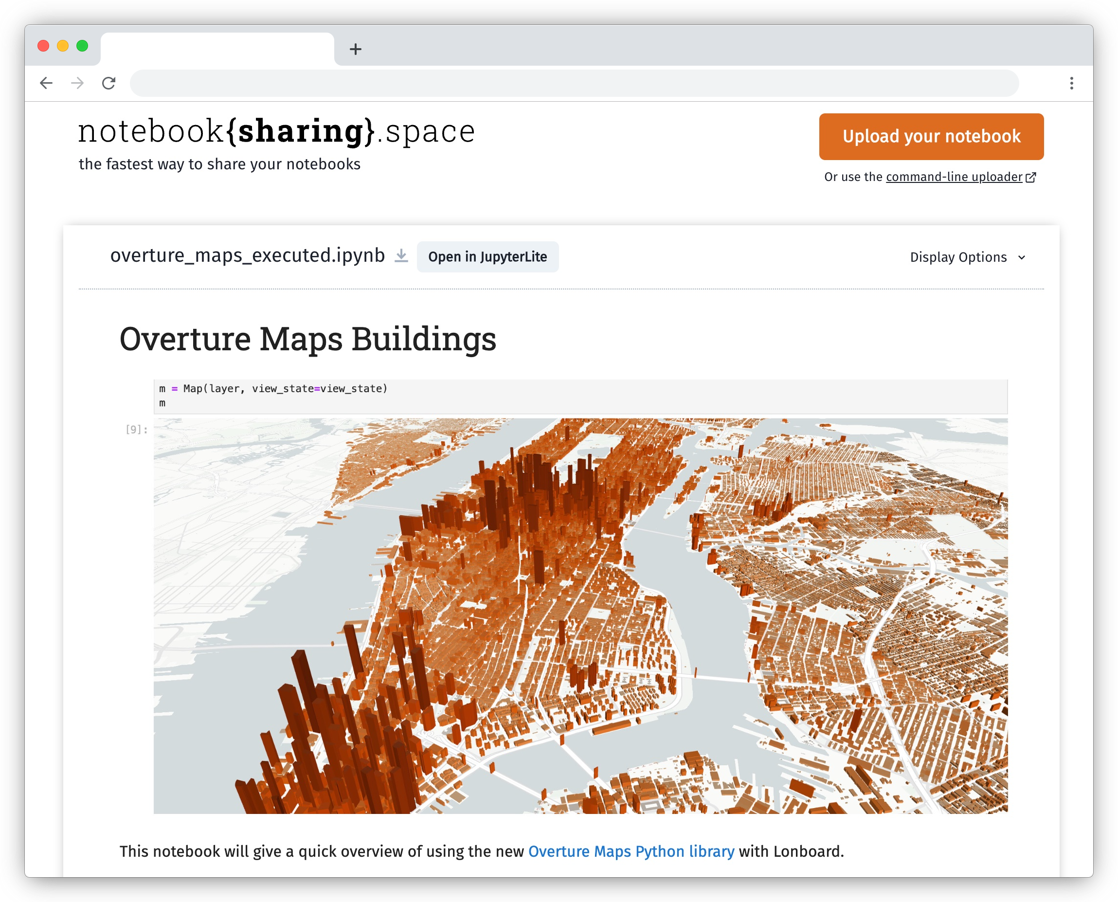
Viewing a notebook published on notebooksharing.space
Improving the Ecosystem through Collaboration
Geospatial data and map visualizations are complicated. While we have moved past static images rendered on the backend to interactive maps on the front end, there’s still a lot we want from the Jupyter ecosystem. Existing map libraries primarily rely on GeoJSON as the interchange and visualization format. This becomes a bottleneck when reading large datasets. Lonboard is solving this performance problem using using GeoArrow and avoiding any serializations to read large volumes of data.
We want maps to become a central element in computation notebooks. It should allow users to filter data to update charts, react based on code changes, and work seamlessly with existing notebook widgets. Our work on Lonboard aims to fill some gaps in the Jupyter ecosystem. And by leveraging eoAPI's cloud-native stack, we're enabling Jupyter to handle large-scale data access efficiently.
Lonboard brings powerful interactive map visualization into Jupyter
Integrating maps as core elements in Jupyter empowers users across skill levels to create impactful visualizations. Data scientists can now publish interactive maps directly from notebook code, eliminating the need to build custom web apps every time you want to share your research.
2i2c is at the forefront of enabling scientific communities with sustainable computing infrastructure based on Jupyter. We are collaborating with them to bring our combined expertise managing large scale EO pipelines and scientific computing to NASA's vision for VEDA which powers platforms like US GHG Center. We are excited to collaborate with QuantStack and Simula on the JupyterGIS project funded by the ESA to push forward the vision of EO data analysis in Jupyter.
If you'd like to talk more about enabling open science in the browser and the latest technologies we are working on, we'll be at ESIP and would love to connect.
What we're doing.
Latest