
Time is in Your Favor: Land Use Modeling with Temporal Data
- Estimated
- 5 min read


For mapping Earth, time is key
The increasing revisit frequency of satellite imagery allows us to view it as a very slow movie of the Earth. Satellites like Sentinel-2 record Earth at 73 frames per year, while Planet Dove satellites capture 365 frames per year. One nice visualization of these data archives is the Google Earth Timelapse project.
However, this data is more than a collection of beautiful pictures. Deep stacks of imagery can be used for in-season crop type classification to monitor agricultural production and estimate tree age to track the status of our forests.
Land use and land cover models are behind this type of map. This kind of model is an analysis performed with satellite imagery. Land cover maps classify every piece of earth into categories such as water, rock, agriculture, and urban areas. National agencies produce large-scale land use and land cover maps such as WorldCover from ESA or the National Land Cover Database from USGS. Development Seed is actively working on PEARL, a tool to create custom versions of land use and land cover maps. Another notable example is the global land cover map produced by Impact Observatory.
The increasing data richness changes the perspective on how land cover and land use models can operate. Instead of relying on a single snapshot, we can take advantage of the temporal dynamics of the Earth's surface to create better models. This applies to land use models and land cover models. These two land classifications are related but not the same. For both, however, the past is informative for what is there now.
For example, distinguishing deciduous from evergreen trees becomes much easier if the model sees the trees in all seasons. The deciduous trees will have a leaf-on and a leaf-off phase that is easily distinguishable. Evergreen trees, on the other hand, will be green all year long! Another example is crop type identification. Different crops are planted at different times of the year and may have different colors when blooming. A model can use these dynamics to learn to differentiate crop types.
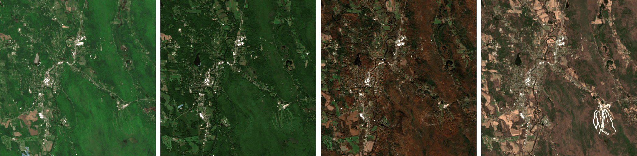
A mix of agricultural areas with deciduous and evergreen forests, illustrating the dynamics for a piece of Massachusetts, USA, between September and November 2022
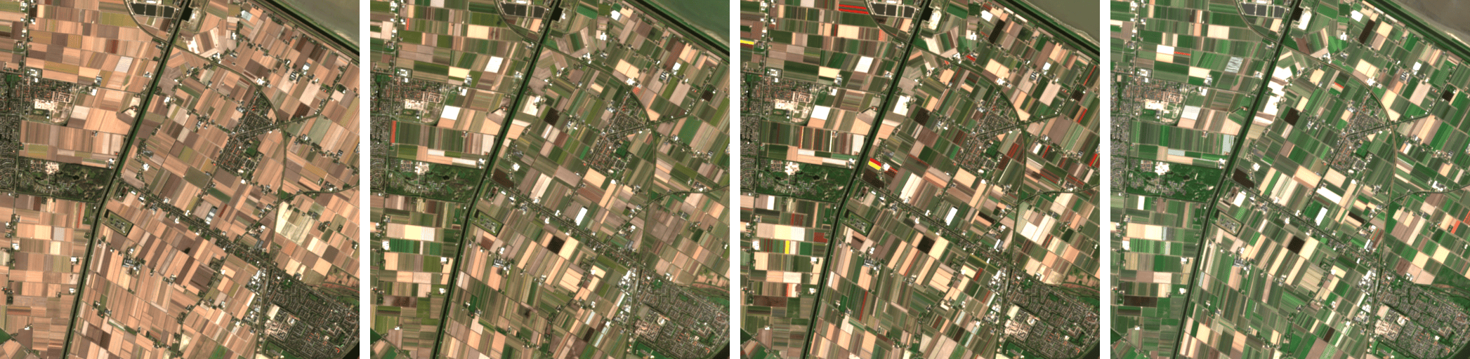
Agricultural fields in the Netherlands between March and June 2022
The additional information available with time series data is essential to model land use accurately. Land use modeling asks the question: what is the use of the land? In many cases, this question can not even be answered with a single satellite image. For instance, in a single image, agricultural land recently plowed is indistinguishable from abandoned land with bare soil. However, a plowed field is still productive and actively used cropland - even after it was plowed. If we obtain information about the plowed field from before plowing, during the crop growth phase, and during the harvest period, there is no doubt that this land is used for agriculture. Modern machine learning models can pick up on that and leverage the additional information for classification.
Land use change is slow
A time series approach to land use modeling works well because, from an earth observation modeling perspective, land use changes slowly. Over the last 60 years, the average global rate of land use change was around 0.5% per year. Given that land cover models are considered acceptable if the accuracy is 80% and excellent if it's above 90%, land use can essentially be regarded as stable for many practical cases. Considering this, we can feed a model months or even years' worth of data to distinguish different types of land use.
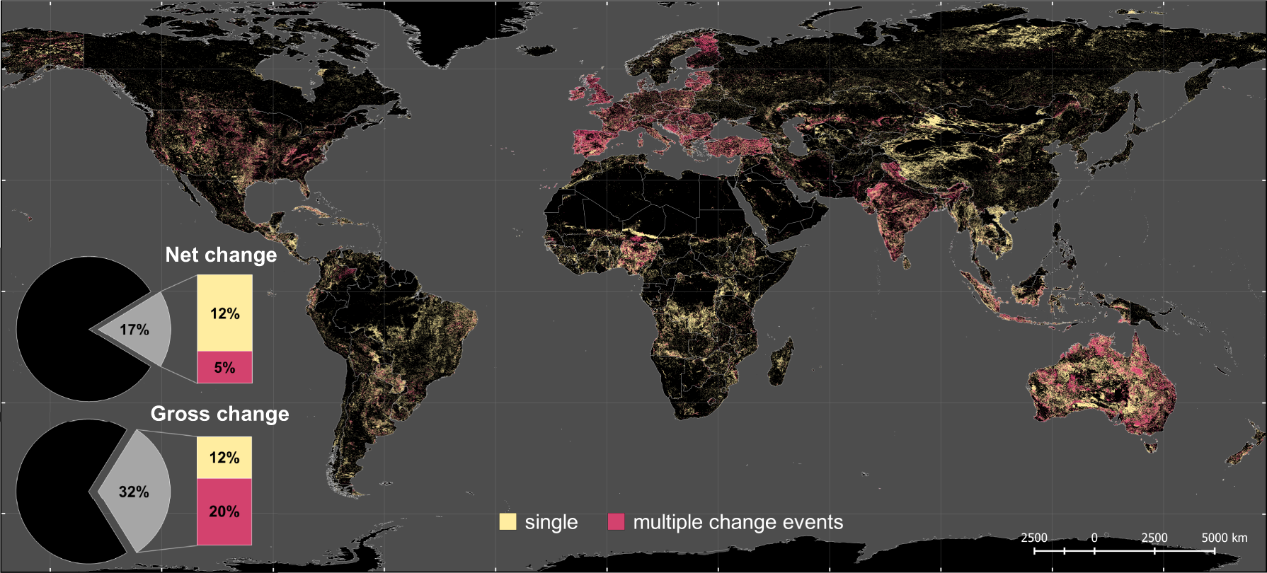
Spatial extent of global land use/cover change. Image from Winkler, K., Fuchs, R., Rounsevell, M. et al. 2021.
Land use change modeling with time series data is an even more challenging problem that requires additional attention. Since land use changes are often small compared to overall areas, change models must focus on that directly. Simply running a land use model over two different years will result in mainly reporting spurious changes. The changes will probably be detected correctly but be buried under a sea of small artifact changes due to the model error.
Smoothing out negative image artifacts
Another good reason to use multiple images is that satellite images are not as clean as you think. We are all used to the perfect Google Maps images, where it is always summer and clouds do not exist. In reality, images can be hazy, have clouds in them, have minor errors in geographic placement (more technically, errors in georeferencing and orthorectification), and have different data distributions due to variations in brightness and contrast because of atmospheric conditions or illumination angles. These random artifacts in satellite imagery are all errors that average over a series of images. Models can learn how to ignore atmospheric effects and clouds and average over errors in geographic image placement. This will make the model robust to these variations and less dependent on the quality of a single image.
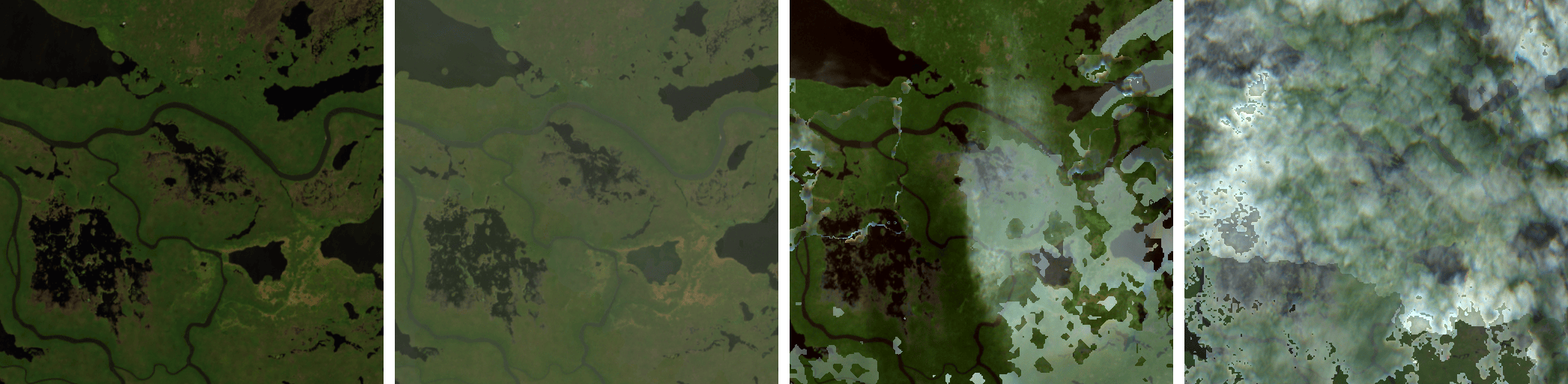
Illustration of varying image quality with different atmospheric effects in image composites for a piece of Sub Saharan Africa between May 2022 and April 2023
Time series are cool. Now what?
We hope we have made a positive case for using time series in land use modeling. In our next blog, we’ll dive deeper into the technical aspects. We’ll summarize some bleeding edge models that use today's time series modeling. And then, we’ll show an example of how this additional dimension can help create better maps faster in real-world use cases. Stay tuned!
What we're doing.
Latest