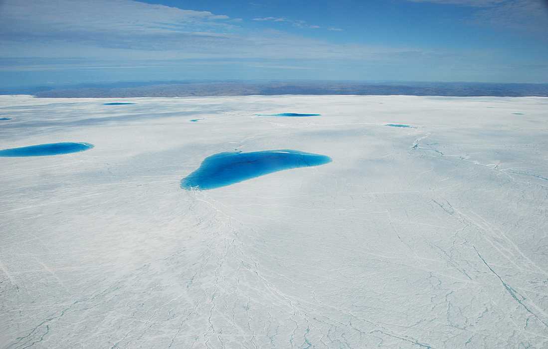
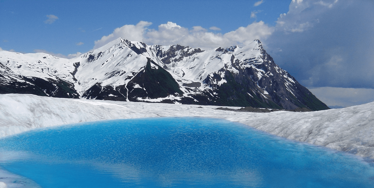
Glaciers are melting fast. Losing ice at the unprecedented rate of 267 ± 16 gigatons per year. This affects regional hydrology around glaciers and global-scale sea level rise (Hugonnet, R., McNabb, R., Berthier, E. et al., 2021). Supraglacial lakes (SGLs) - a pond or pool that forms on top of a glacier - play a fundamental role in the functioning of ice sheets. Their formation contributes to a warming effect on ice sheets. SGLs have a lower albedo - surface reflectance - than ice, absorbing more heat from the sun. Scientists have been studying and tracking SGLs in the Arctic to understand the impact of SGLs on ice sheet health or change.
Historically, satellite detection of SGLs was limited due to the variability in the scale of SGL extent and frequent cloud coverage of the Arctic during the summer. Constellations of low earth-orbiting satellites such as PlanetScope offer the potential to frequently monitor these broad scales with frequency and granularity (Arthur et al., 2020).
Most measurements and characterization of SGLs and corresponding sea ice albedo evolution derive from in situ studies. Remote sensing observations provide the best current data to understand SGLs and albedo changes on a scale broad enough to infer systemic changes. Many sensors' spatial and temporal constraints are reducible with imagery from small satellite systems, such as the PlanetScope constellation, which feature high revisit rates and spatial resolution (Arthur et al., 2020).
Supraglacial lakes (SGLs), also known as melt ponds, result from meltwater accumulation in topographic depressions on the surface of glaciers, primarily occurring during the ablation season. SGLs affect ice sheet dynamics through a positive feedback loop in which the albedo-lowering effect of SGLs can escalate surface melt. This effect increases lake extent and depth, amplifying the albedo-lowering effect. Fluctuations in SGLs over time can induce ice flexure and fracturing, enabling mechanisms for meltwater to enter and affect the interior of the ice sheet (Arthur et al., 2020). The implications of accelerated glacial melt include increased sea level rise and modifications to ocean productivity (Robel et al., 2019; Horvat et al., 2017).
The implications of accelerated glacial melt include increased sea level rise and modifications to ocean productivity.
Efficient monitoring of SGLs is critical. They are indicators of surface melt and its associated downstream impacts. Earth remote sensing observation data and machine learning enable scalable monitoring of SGLs through pattern detection and quantification of lake evolution over time (Arthur et al., 2020; Hochreuther et al., 2021; Lee, 2020). On-site observations and measurements of SGLs are time-consuming, cost-prohibitive, and challenging to achieve at scale. (Lee, 2020). Small satellite imagery with high temporal and relatively high spatial resolution offers the potential to closely monitor dynamic changes in SGL formation, drainage, and associated impacts on ice shelves (Arthur et al., 2020).
This work developed an approach using supervised semantic segmentation leveraging a convolutional neural network architecture to train a model with imagery and labels from NASA Operation IceBridge and predict SGL occurrences in high temporal resolution PlanetScope imagery. We chose this approach to enable rapid prototyping of a model without the need for manually creating labels ourselves. Currently, NASA Operation IceBridge provides our best option for pre-existing labels representing SGLs, our feature of interest. Co-locating PlanetScope imagery with the IceBridge labels presented a challenge due to the unknown ortho-rectification techniques of the labels. We chose to use the labels with their original imagery. We applied pre-processing to enable the IceBridge imagery to simulate PlanetScope.
Our segmentation model was built upon the Unet architecture and was pre-trained with a mobilenetv2 backbone. We computed the F1 score, Intersection over Union (IoU) score, total accuracy, and confusion matrices to evaluate our model.
Data Processing
Our data processing and analysis were different for training and inference. We utilized IceBridge for training and PlanetScope for inference. Both datasets, however, were evaluated for model performance.
IceBridge dataset processing and analysis
The IceBridge campaign entails a multi-year archive of 10-centimeter aerial imagery with visual wavelengths over polar regions. Several years' worth of IceBridge data has associated segmentation labels available derived from another machine learning approach (Wright & Polashenski, 2018).
To constrain the focus of our model, the training data we acquired from the IceBridge archive covered four dates worth of data over 2015-2016 and was selected from Arctic regions to study several ice shelves in the North Atlantic (as indicated in the plot below).

This plot indicates time and space-bound PlanetScope imagery coverage of several areas of interest.
Once the IceBridge scenes were acquired, we established a workflow to downsample each scene to approximate the spatial resolution of PlanetScope imagery (our inference target). Tiling at uniform image width and height dimensions for use in a machine learning workflow followed.
The labels had six classes: no data, snow and bright ice, dark and thin ice, melt ponds and submerged ice, open water, and ridge shadows. The last class was sparsely represented and dropped from the modeling objective. It would have been ideal to have a class for exposed rock, as this often presents in some areas within and along the ice shelves. The model was not given instructions to account for these features.
As stated, the labels were derived from another machine learning approach. Expectedly, they inherit some errors. The metadata for each scene includes a quality score; however, even at the highest quality score, there was a non-trivial amount of error in the labels. We sought to account for the bulk of misclassifications by doing a manual quality assurance (QA) check to remove highly erroneous scenes.
After QA, the dataset was partitioned into training, validation, and test sets with a 70:20:10 percent ratio. Reasonable stratification of classes and timestamps was checked for across the partitions.
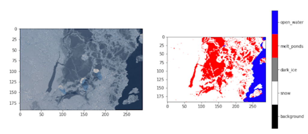
Sample IceBridge scene and associated raster label.
PlanetScope
For PlanetScope, we used the analytic surface reflectance product, which produces a better signal of SGLs in its true color representation. It also includes the near-infrared channel, which comes in handy when weeding out false positives.
Process-wise, the true color images are created, tiled (to the exact image dimensions as the IceBridge training tiles), and segmented by our trained model. The near-infrared channel is tiled and used after inference for filtering false positives in the melt pond class predictions. As previously mentioned, exposed rock presents a false positive for water features (melt pond and open water). None of the label classes account for exposed rock, even though it is a common feature across ice shelves. We successfully leveraged a combination of near-infrared, NDWI, and blue channel thresholding to filter out false positives of this type (more on this later).
Results
IceBridge
We reserved 10% of the IceBridge tiled training data for testing. Our model was evaluated in two ways: 1) tile-wise and 2) randomly sampled pixel-wise (1000 pixels) across the 20 Icebridge scenes in the test partition. This latter evaluation was done to compare with the results in the research which produced the original labels (Wright & Polashenski, 2018).
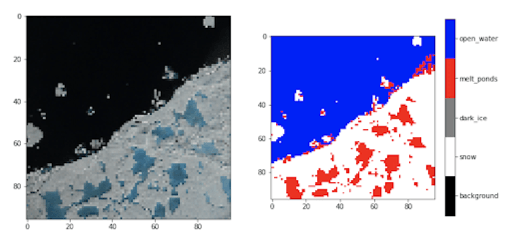
Sample IceBridge tile and associated model segmentation inference.
For the confusion matrices proceeding here, class 0 = background, class 1 = snow/bright ice, class 2 = dark and thin ice, class 3 = melt pond/SGL, and class 4 = open water.
Tile-wise evaluation
The overall F1 and IoU scores (positive classes only) for the test partition of the IceBridge dataset are 0.62 and 0.49, respectively.
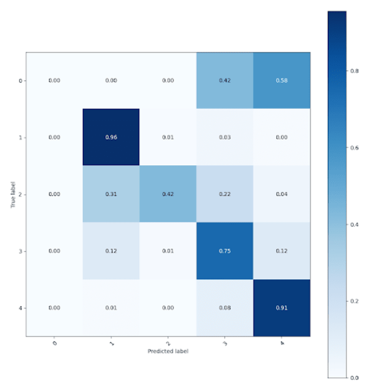
Normalized confusion matrix based on the IceBridge test tiles.
Pixel-wise (randomly sampled) evaluation
An evaluation of 1000 randomly sampled pixels across 20 IceBridge images from the test partition where only pixels with values > 0 were sampled. The evaluation of our model produced an overall accuracy over the four positive classes (snow and ice, dark ice, melt pond, and open water), equaling 90%.
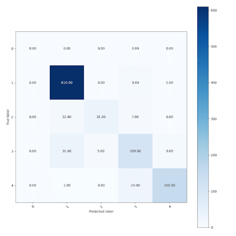
Absolute count confusion matrix based on 1000 randomly sampled pixels from the IceBridge test tiles.
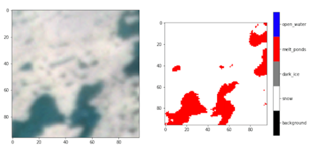
Sample PlanetScope tile and associated model segmentation inference. Includes copyrighted material of Planet. All rights reserved.
Tile-wise evaluation
The overall F1 and IoU scores (positive classes only) for the test partition of the IceBridge dataset are 0.52 and 0.32, respectively.
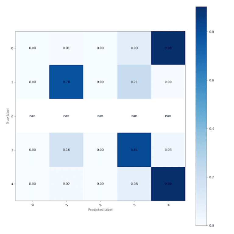
Normalized confusion matrix based on the PlanetScope test tiles.
Pixel-wise (randomly sampled) evaluation
An evaluation of 1000 pixels randomly sampled across ten manually annotated PlanetScope image tiles where only pixels with values > 0. The evaluation of our model produced an overall accuracy over the four positive classes (snow and ice, dark ice, melt pond, and open water), equaling 75%.
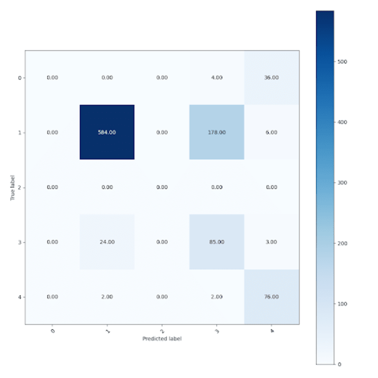
Absolute count confusion matrix based on 1000 randomly sampled pixels from the PlanetScope test tiles.
Discussion
The confusion between melt ponds and snow/bright ice pixels in this confusion matrix may be due to the complexity of accurately delineating and labeling melt ponds, particularly when found in fragmented networks. Take the following PlanetScope image tile as an example of a relevant difficult annotation task. Many melt pond pixels are hard to annotate correctly and entirely in the labeling process.
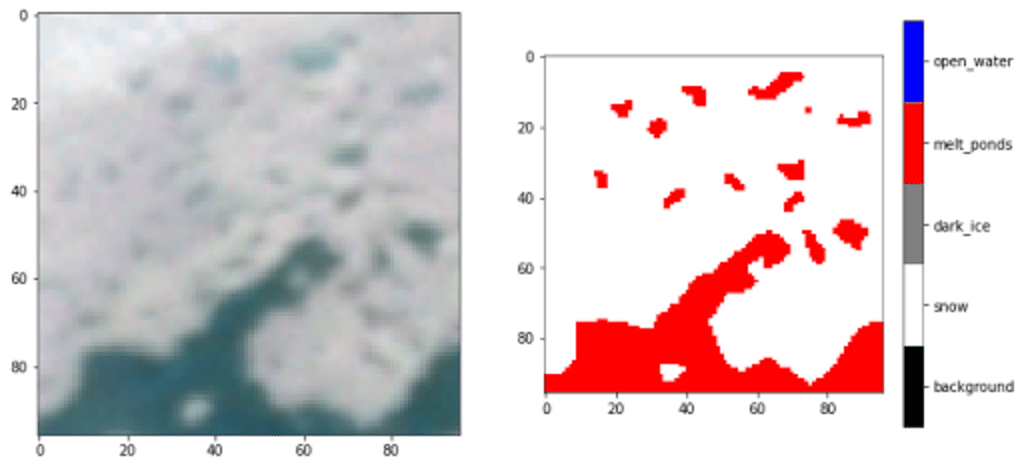
PlanetScope manually annotated tile example. Includes copyrighted material of Planet. All rights reserved.
The current methods to remove false positive pixels using the Normalized Difference Water Index, near-infrared channel, and blue channel do a decent job but are not perfect solutions (see below).
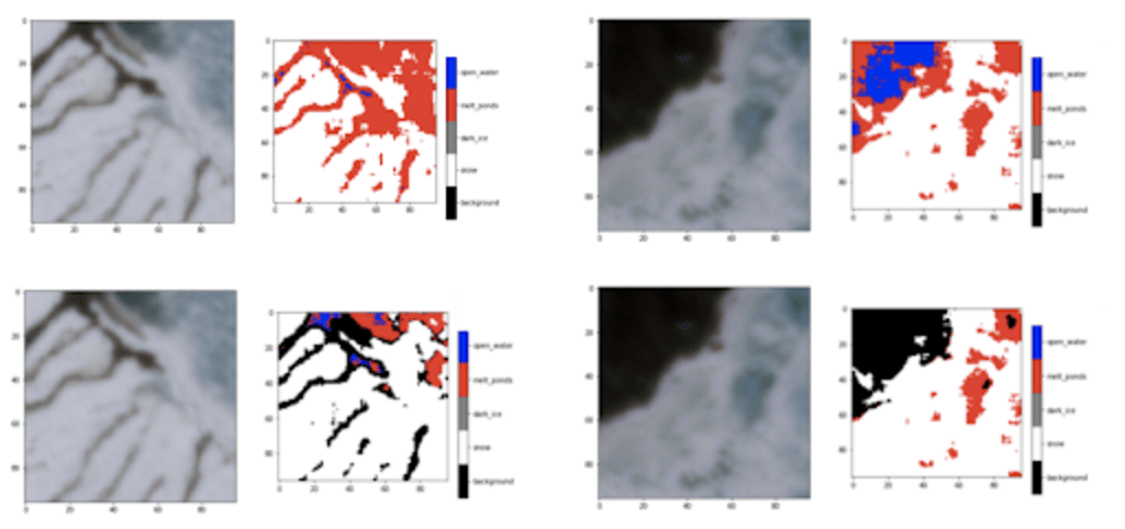
Exposed rock false positive filtering (black pixels are masked result). Includes copyrighted material of Planet. All rights reserved.
After talking with NASA cryosphere scientists, a future idea is to leverage digital elevation models (DEMs) to remove high terrain melt pond pixels, which we expect to show true positives to exist in topographic depressions.
Conclusion
Having completed the initial discovery phase of this research, we are now discussing methods to improve our model with subject matter experts in the cryosphere domain. We hope the publication of an ML dataset and paper will follow this. The code repository is at https://github.com/NASA-IMPACT/veda-ai-supraglacial_segmentation.
We hope that by sharing our approach to detecting, measuring, and monitoring SGLs, others may build upon this to further improve the observation of these features and their effects on the climate. We want to encourage cryosphere scientists with expertise in SGLs to use ML in their research wherever it may be helpful. We hope that in proving the scalability, cost-efficiency, and accuracy of combined ML and EO, both may become more instrumental in studying these geographically hard-to-access features.
We hope that others may build upon this approach to further improve the observation of these features and their effects on the climate.
We seek feedback on our methods and ideas for improvement from the community. We also want to know how we may further help others study SGLs and their impact. Our goal is to add to this domain's knowledge pool and provide additional ways to derive insights.
We would like to acknowledge Planet and the NASA Commercial Smallsat Data Acquisition Program (CSDA) for provisioning data and NASA Marshall Space Flight Center for funding this research.
To get in touch to discuss this project or provide feedback, reach out to Lilly at @lilly_e_thomas.
Citations
Arthur, J. F., Stokes, C., Jamieson, S. S., Carr, J. R., & Leeson, A. A. (2020). Recent understanding of Antarctic supraglacial lakes using satellite remote sensing. Progress in Physical Geography: Earth and Environment, 44(6), 837–869. https://doi.org/10.1177/0309133320916114
C. Horvat et al. The frequency and extent of sub-ice phytoplankton blooms in the Arctic Ocean [J] Sci. Adv. (2017)
Hochreuther, P.; Neckel, N.; Reimann, N.; Humbert, A.; Braun, M. Fully Automated Detection of Supraglacial Lake Area for Northeast Greenland Using Sentinel-2 Time-Series. Remote Sens. 2021, 13, 205. https://doi.org/10.3390/rs13020205
Hugonnet, R., McNabb, R., Berthier, E. et al. Accelerated global glacier mass loss in the early twenty-first century. Nature 592, 726–731 (2021). https://doi.org/10.1038/s41586-021-03436-z
Robel, A. A., & Banwell, A. F. (2019). A speed limit on ice shelf collapse through hydrofracture. Geophysical Research Letters, 46, 12092– 12100. https://doi.org/10.1029/2019GL084397
S. Lee et al. Machine learning approaches to retrieve pan-Arctic melt ponds from visible satellite imagery [J] Remote Sens. Environ. (2020)
What we're doing.
Latest

