
Table of Contents
Setup
%%time
import os
from pathlib import Path

data_dir = Path("data")

try:
    import google.colab
    IN_COLAB = True
except:
    IN_COLAB = False

if IN_COLAB:
    # Mount drive to access data
    from google.colab import drive
    drive.mount('/content/drive')

    !pip install uv
    !uv pip install --system \
        "adlfs==2024.7.0" \
        "dask==2024.11.2" \
        "fsspec==2024.10.0" \
        "geopandas==1.0.1" \
        "matplotlib==3.9.2" \
        "numcodecs==0.15.1" \
        "planetary-computer==1.0.0" \
        "pyarrow==18.0.0" \
        "pystac-client==0.8.5" \
        "xarray==2024.11.0" \
        "zarr==2.18.3" \
        "odc-stac==0.3.10" \
        "rasterio==1.4.2" \
        "rioxarray==0.18.1" \
        "rasterstats==0.20.0" \
        "numpy==2.1.3"

    data_dir = Path("/content/drive/MyDrive/earthsense25tutorial")

    print("✅ Environment activated and data ready!")
Note: In Colab, restart the runtime after installing the packages to ensure all the packages are loaded.
Introduction
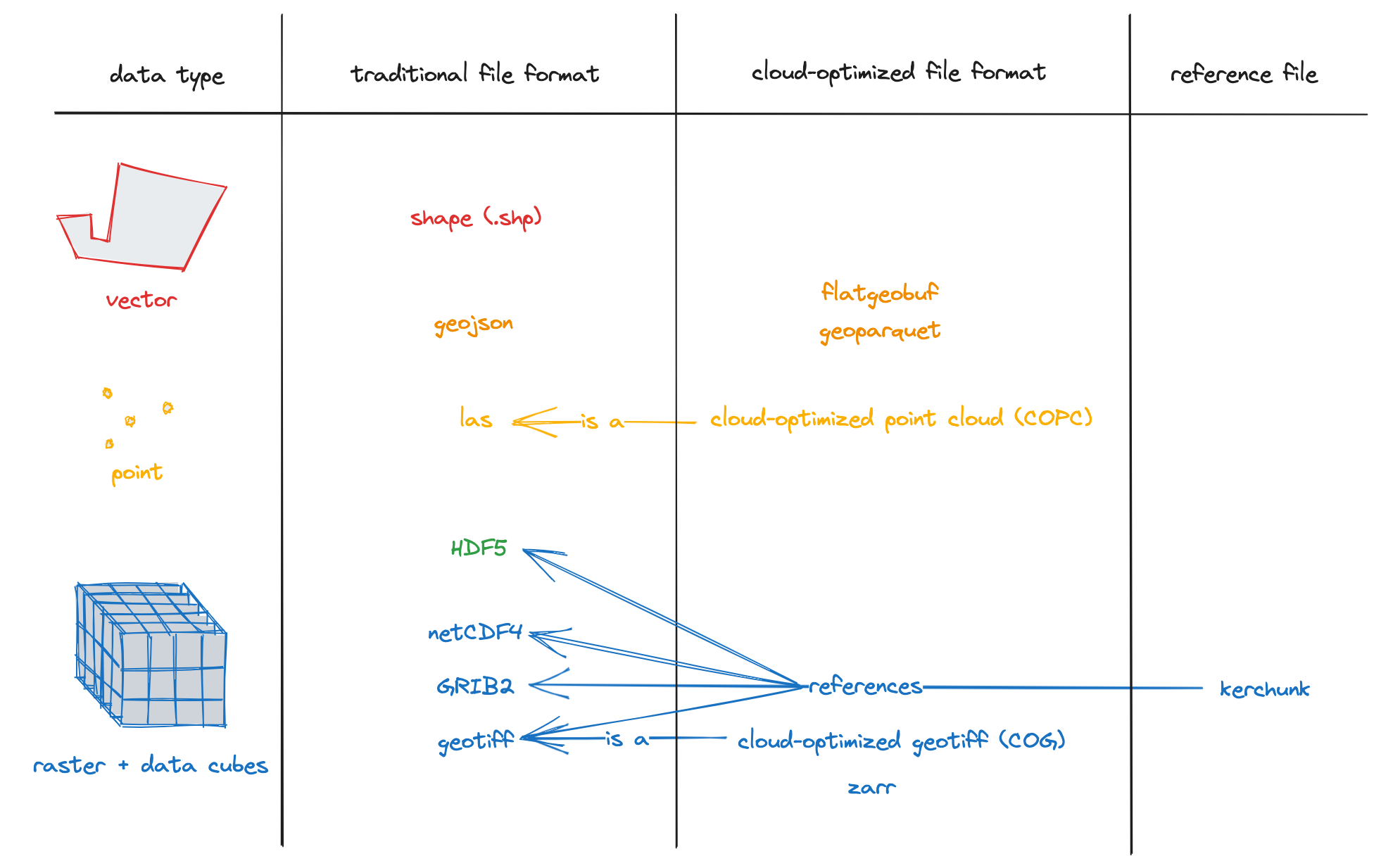
Geospatial data comes in many unique formats - including rasters, vectors, and point clouds. With the rapid growth of data sources like satellites, drones, and sensors, both the volume and complexity of geospatial data continues to increase exponentially.
To handle this data efficiently at scale, the community has developed Cloud Native data formats. These formats are specifically designed for cloud-based storage and processing.
Key characteristics of Cloud Native Data Formats:
Optimized for reading operations
Support for parallel reads from multiple processes/threads
Ability to read specific subsets of data without loading entire files
Fast metadata access in a single operation
Internal organization into tiles and chunks for efficient data access
Compatible with HTTP range requests for efficient access from cloud storage
Please check this guide made by our amazing colleagues at Development Seed to learn more: https://
Cloud Native Data Formats
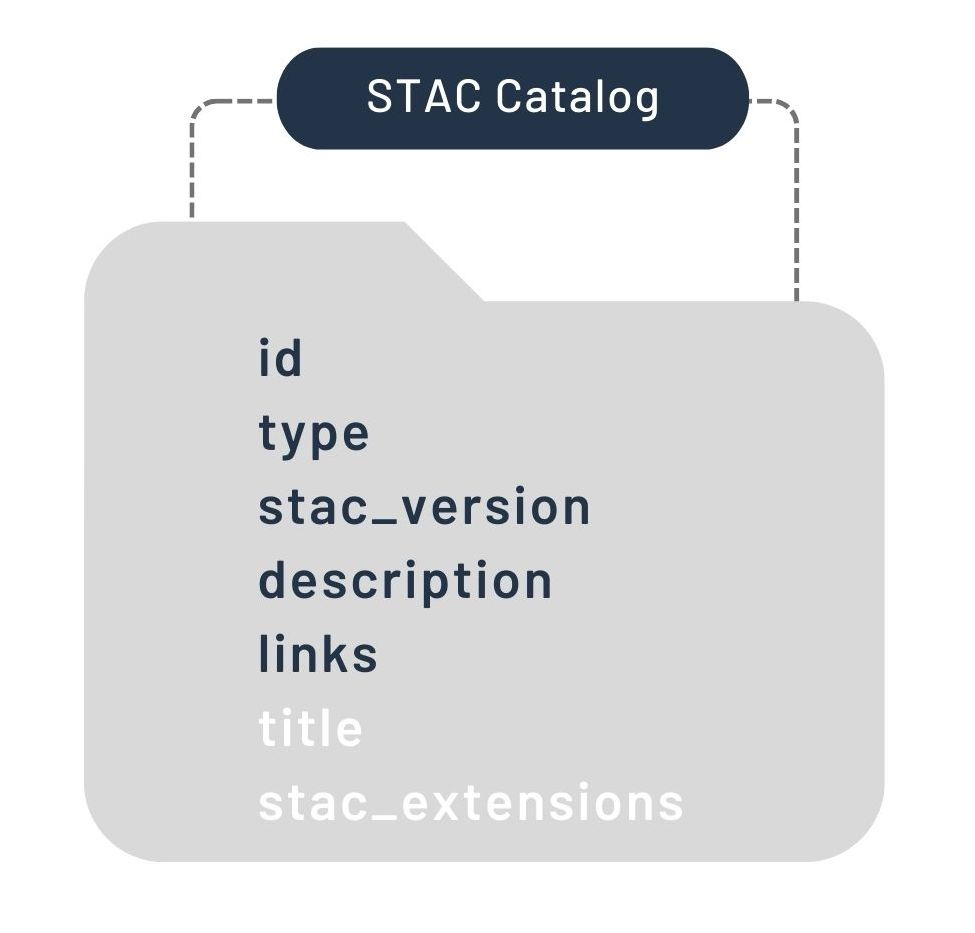
SpatioTemporal Asset Catalog (STAC)
The SpatioTemporal Asset Catalog (STAC) is a standard for describing geospatial datasets in a consistent and searchable manner. It defines a common structure for cataloging spatial and temporal metadata, enabling easy discovery and access to geospatial assets.
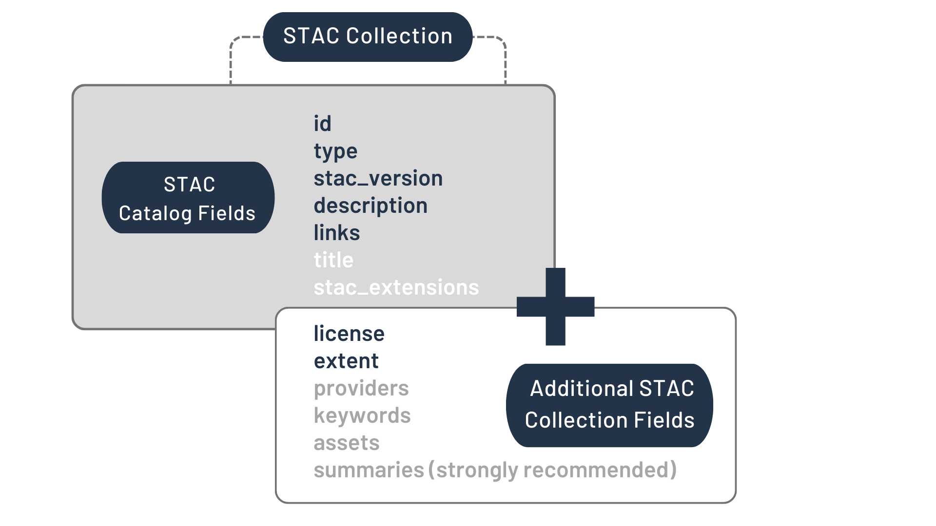
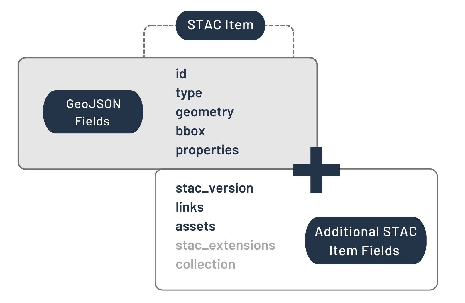
STAC is organized into:
Catalogs: Hierarchical grouping of Collections and Items.
Collections: Groups of Items with shared metadata.
Items: Individual geospatial assets with metadata.
STAC Index - https://
STAC Browser - https://
Cloud Optimized GeoTIFFs (COGs)
Cloud Optimized GeoTIFFs (COGs) are GeoTIFF files structured in a way that makes it possible to efficiently stream subsets of imagery data, enabling fast and scalable data retrieval.
Key features of COGs:
Internal tiling for efficient read access.
Compatibility with HTTP range requests, so they can be stored in object storage & supports parallel/partial reads
Pairs well with STAC to index & serve data
Used to store raster data that represent a snapshot in time or limited assets. Satellite Imagery, DEM, etc

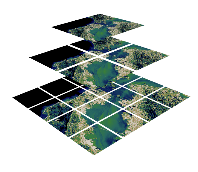
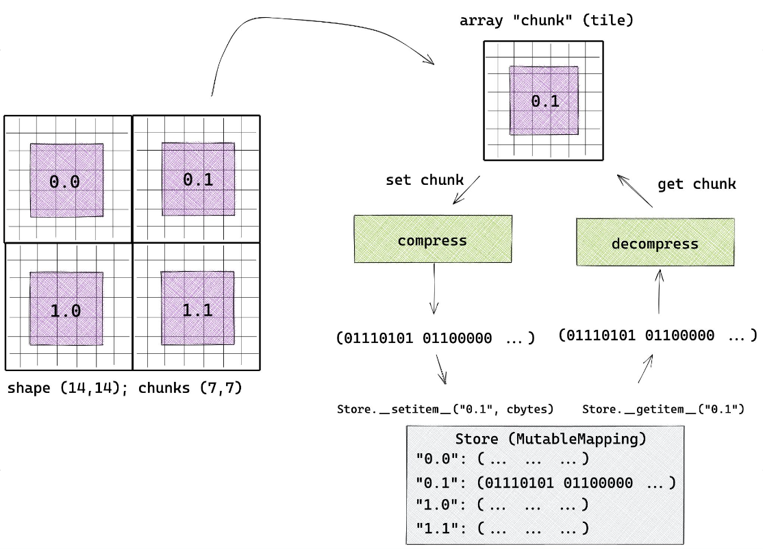
Zarr
Zarr is a format for the storage of chunked, compressed, N-dimensional arrays. It is ideal for large-scale, multi-dimensional datasets, such as weather data, climate models, and hyperspectral imagery.
Key features of Zarr:
Supports chunking and compression for efficient storage and access.
Metadata is store independently of the chunked data, facilitating efficient read access
Supports parallel and partial reads, making it suitable for cloud storage and processing
Used to store multi-dimensional rasters or datacubes. Weather data, Climate Models, Time-series data, Satellite Imagery, etc
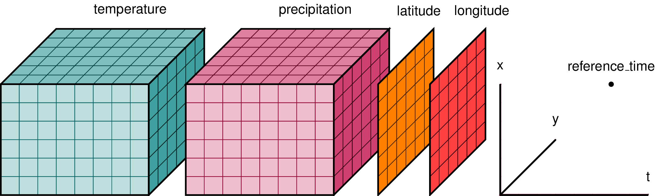
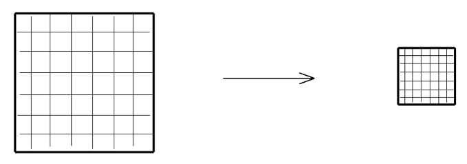
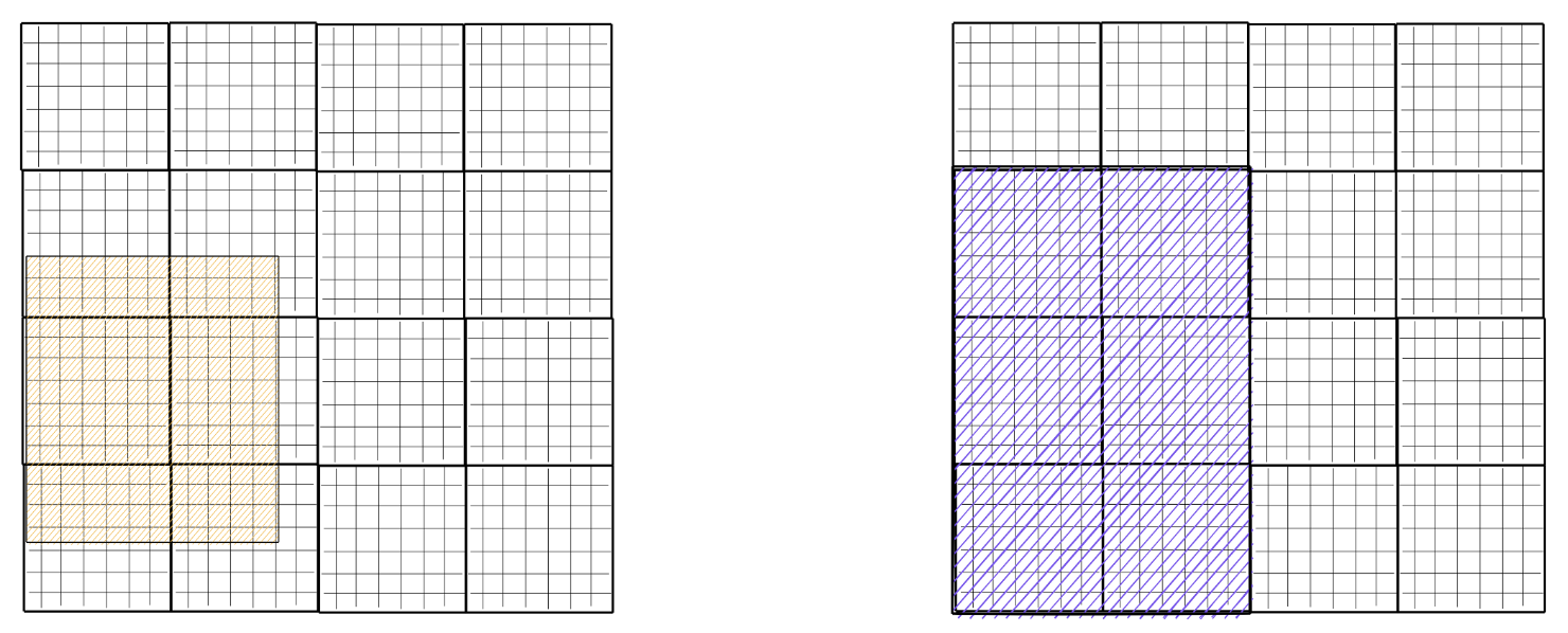
How Zarr works?
thanks to Sanket Verma for his amazing slides on Zarr - the following images are taken from his presentation

Analyzing ERA5 Reanalysis Data
In this tutorial, we will:
Parse a STAC catalog to discover data assets.
Read ERA5 reanalysis data stored in Zarr format.
Visualize the data and create animations.
Create time-series plots and perform data analysis.
Parsing the STAC Catalog
We will use the pystac-client library to interact with the STAC catalog and discover ERA5 reanalysis data.
ECMWF Reanalysis Data (ERA5)
ERA5 is the fifth generation ECMWF atmospheric reanalysis of the global climate covering the period from January 1940 to present. ERA5 is produced by the Copernicus Climate Change Service (C3S) at ECMWF.
ERA5 provides hourly estimates of a large number of atmospheric, land and oceanic climate variables. The data cover the Earth on a 31km grid and resolve the atmosphere using 137 levels from the surface up to a height of 80km. ERA5 includes information about uncertainties for all variables at reduced spatial and temporal resolutions.
import pystac_client
from datetime import datetime
import planetary_computer

# Initialize the STAC client
catalog = pystac_client.Client.open(
    "https://planetarycomputer.microsoft.com/api/stac/v1/"
)
Let’s explore a few collections available in the catalog.
# List the first 10 collections
for collection in list(catalog.get_collections())[:10]:
    print("Name: ", collection.title)
    print("ID: ", collection.id)
    print("-"*50)
Name: Daymet Annual Puerto Rico
ID: daymet-annual-pr
--------------------------------------------------
Name: Daymet Daily Hawaii
ID: daymet-daily-hi
--------------------------------------------------
Name: USGS 3DEP Seamless DEMs
ID: 3dep-seamless
--------------------------------------------------
Name: USGS 3DEP Lidar Digital Surface Model
ID: 3dep-lidar-dsm
--------------------------------------------------
Name: Forest Inventory and Analysis
ID: fia
--------------------------------------------------
Name: Sentinel 1 Radiometrically Terrain Corrected (RTC)
ID: sentinel-1-rtc
--------------------------------------------------
Name: gridMET
ID: gridmet
--------------------------------------------------
Name: Daymet Annual North America
ID: daymet-annual-na
--------------------------------------------------
Name: Daymet Monthly North America
ID: daymet-monthly-na
--------------------------------------------------
Name: Daymet Annual Hawaii
ID: daymet-annual-hi
--------------------------------------------------
We are interested in the ERA5 collection. Lets look at the summary of the collection.
# Find the ERA5 collection
for collection in catalog.get_collections():
    if 'era5' in collection.id.lower():
        print("Name: ", collection.title)
        print("ID: ", collection.id)
        print("Summary: ", collection.summaries.to_dict())
        print("Assets: ", collection.assets)
        print("Extent: ", collection.extent.to_dict())
        print("Description: ", collection.description)
        print("-"*50)
Name: ERA5 - PDS
ID: era5-pds
Summary: {'era5:kind': ['fc', 'an']}
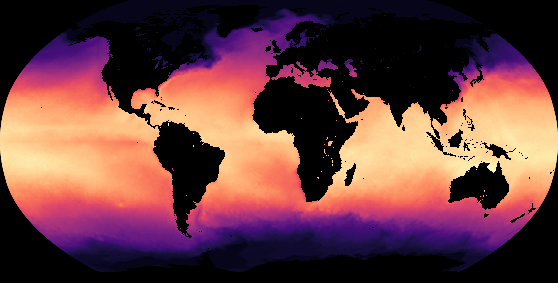
Assets: {'thumbnail': <Asset href=https://ai4edatasetspublicassets.blob.core.windows.net/assets/pc_thumbnails/era5-thumbnail.png>, 'geoparquet-items': <Asset href=abfs://items/era5-pds.parquet>}
Extent: {'spatial': {'bbox': [[-180, -90, 180, 90]]}, 'temporal': {'interval': [['1979-01-01T00:00:00Z', None]]}}
Description: ERA5 is the fifth generation ECMWF atmospheric reanalysis of the global climate
covering the period from January 1950 to present. ERA5 is produced by the
Copernicus Climate Change Service (C3S) at ECMWF.
Reanalysis combines model data with observations from across the world into a
globally complete and consistent dataset using the laws of physics. This
principle, called data assimilation, is based on the method used by numerical
weather prediction centres, where every so many hours (12 hours at ECMWF) a
previous forecast is combined with newly available observations in an optimal
way to produce a new best estimate of the state of the atmosphere, called
analysis, from which an updated, improved forecast is issued. Reanalysis works
in the same way, but at reduced resolution to allow for the provision of a
dataset spanning back several decades. Reanalysis does not have the constraint
of issuing timely forecasts, so there is more time to collect observations, and
when going further back in time, to allow for the ingestion of improved versions
of the original observations, which all benefit the quality of the reanalysis
product.
This dataset was converted to Zarr by [Planet OS](https://planetos.com/).
See [their documentation](https://github.com/planet-os/notebooks/blob/master/aws/era5-pds.md)
for more.
## STAC Metadata
Two types of data variables are provided: "forecast" (`fc`) and "analysis" (`an`).
* An **analysis**, of the atmospheric conditions, is a blend of observations
with a previous forecast. An analysis can only provide
[instantaneous](https://confluence.ecmwf.int/display/CKB/Model+grid+box+and+time+step)
parameters (parameters valid at a specific time, e.g temperature at 12:00),
but not accumulated parameters, mean rates or min/max parameters.
* A **forecast** starts with an analysis at a specific time (the 'initialization
time'), and a model computes the atmospheric conditions for a number of
'forecast steps', at increasing 'validity times', into the future. A forecast
can provide
[instantaneous](https://confluence.ecmwf.int/display/CKB/Model+grid+box+and+time+step)
parameters, accumulated parameters, mean rates, and min/max parameters.
Each [STAC](https://stacspec.org/) item in this collection covers a single month
and the entire globe. There are two STAC items per month, one for each type of data
variable (`fc` and `an`). The STAC items include an `ecmwf:kind` properties to
indicate which kind of variables that STAC item catalogs.
## How to acknowledge, cite and refer to ERA5
All users of data on the Climate Data Store (CDS) disks (using either the web interface or the CDS API) must provide clear and visible attribution to the Copernicus programme and are asked to cite and reference the dataset provider:
Acknowledge according to the [licence to use Copernicus Products](https://cds.climate.copernicus.eu/api/v2/terms/static/licence-to-use-copernicus-products.pdf).
Cite each dataset used as indicated on the relevant CDS entries (see link to "Citation" under References on the Overview page of the dataset entry).
Throughout the content of your publication, the dataset used is referred to as Author (YYYY).
The 3-steps procedure above is illustrated with this example: [Use Case 2: ERA5 hourly data on single levels from 1979 to present](https://confluence.ecmwf.int/display/CKB/Use+Case+2%3A+ERA5+hourly+data+on+single+levels+from+1979+to+present).
For complete details, please refer to [How to acknowledge and cite a Climate Data Store (CDS) catalogue entry and the data published as part of it](https://confluence.ecmwf.int/display/CKB/How+to+acknowledge+and+cite+a+Climate+Data+Store+%28CDS%29+catalogue+entry+and+the+data+published+as+part+of+it).
--------------------------------------------------
Reading and Processing Zarr Data
We will query the ERA5 collection for data over India during the Kharif season (June to November 2020). We will filter the data based on a bounding box and temporal range.
import xarray as xr

# Bounding box for India [min_lon, min_lat, max_lon, max_lat]
india_bbox = [68.1, 6.5, 97.4, 37.1]

# Temporal range for Kharif Season
datetime_range = "2020-06-01/2020-11-30"

# Search parameters
search = catalog.search(
    collections=["era5-pds"],
    bbox=india_bbox,
    datetime=datetime_range,
    query={
        "era5:kind": {
            "eq": "an"  # Filter for analysis data only
        },
    }
)

# Fetch matching items
items = search.item_collection()
print(f"Number of matching items: {len(items)}")
Number of matching items: 6
Lets inspect the items from the collection
for item in items:
    print("Item ID:", item.id)
    print("Available assets:", list(item.assets.keys()))
    print("-"*50)
Item ID: era5-pds-2020-11-an
Available assets: ['surface_air_pressure', 'sea_surface_temperature', 'eastward_wind_at_10_metres', 'air_temperature_at_2_metres', 'eastward_wind_at_100_metres', 'northward_wind_at_10_metres', 'northward_wind_at_100_metres', 'air_pressure_at_mean_sea_level', 'dew_point_temperature_at_2_metres']
--------------------------------------------------
Item ID: era5-pds-2020-10-an
Available assets: ['surface_air_pressure', 'sea_surface_temperature', 'eastward_wind_at_10_metres', 'air_temperature_at_2_metres', 'eastward_wind_at_100_metres', 'northward_wind_at_10_metres', 'northward_wind_at_100_metres', 'air_pressure_at_mean_sea_level', 'dew_point_temperature_at_2_metres']
--------------------------------------------------
Item ID: era5-pds-2020-09-an
Available assets: ['surface_air_pressure', 'sea_surface_temperature', 'eastward_wind_at_10_metres', 'air_temperature_at_2_metres', 'eastward_wind_at_100_metres', 'northward_wind_at_10_metres', 'northward_wind_at_100_metres', 'air_pressure_at_mean_sea_level', 'dew_point_temperature_at_2_metres']
--------------------------------------------------
Item ID: era5-pds-2020-08-an
Available assets: ['surface_air_pressure', 'sea_surface_temperature', 'eastward_wind_at_10_metres', 'air_temperature_at_2_metres', 'eastward_wind_at_100_metres', 'northward_wind_at_10_metres', 'northward_wind_at_100_metres', 'air_pressure_at_mean_sea_level', 'dew_point_temperature_at_2_metres']
--------------------------------------------------
Item ID: era5-pds-2020-07-an
Available assets: ['surface_air_pressure', 'sea_surface_temperature', 'eastward_wind_at_10_metres', 'air_temperature_at_2_metres', 'eastward_wind_at_100_metres', 'northward_wind_at_10_metres', 'northward_wind_at_100_metres', 'air_pressure_at_mean_sea_level', 'dew_point_temperature_at_2_metres']
--------------------------------------------------
Item ID: era5-pds-2020-06-an
Available assets: ['surface_air_pressure', 'sea_surface_temperature', 'eastward_wind_at_10_metres', 'air_temperature_at_2_metres', 'eastward_wind_at_100_metres', 'northward_wind_at_10_metres', 'northward_wind_at_100_metres', 'air_pressure_at_mean_sea_level', 'dew_point_temperature_at_2_metres']
--------------------------------------------------
# Sort the items by month
items = list(reversed(items))
We will select the air_temperature_at_2_metres asset for further analysis.
# Select the June item and asset
june_item = items[0]
june_air_temp_asset = june_item.assets["air_temperature_at_2_metres"]

# Sign the asset URL for authentication
june_air_temp_asset = planetary_computer.sign(june_air_temp_asset)

# Display the asset
june_air_temp_assetNow, we can open the asset as an xarray dataset.
%%time
# Open the dataset
june_ds = xr.open_dataset(
    june_air_temp_asset.href,
    **june_air_temp_asset.extra_fields["xarray:open_kwargs"]
)
june_ds.air_temperature_at_2_metresjune_ds.dimsFrozenMappingWarningOnValuesAccess({'time': 720, 'lat': 721, 'lon': 1440})We can filter the data based on the latitude and longitude to cover only India.
# Filter the data to cover only India
june_ds = june_ds.sel(lat=slice(37, 8), lon=slice(67, 100))
june_ds.air_temperature_at_2_metresNote: All the operations are lazy in xarray, so the data is not loaded into memory yet. We need to call the compute() method to load the data into memory.
Let’s compute the data.
%%time
june_ds = june_ds.compute()
june_ds.air_temperature_at_2_metres
# Save the data to a Zarr store
june_ds.to_zarr(f"{data_dir}/june_air_temperature.zarr")
june_ds = xr.open_zarr(f"{data_dir}/june_air_temperature.zarr")june_ds.air_temperature_at_2_metresVisualizing Temperature Data
Calculating Daily Mean Temperature
We will calculate the daily mean temperature for June 2020 over India.
# calculate daily mean
june_daily_mean = june_ds.air_temperature_at_2_metres.resample(time='1D').mean()
Converting Temperature to Celsius
# Convert from Kelvin to Celsius
june_daily_mean_celsius = june_daily_mean - 273.15
Plotting Temperature on a Specific Day
import matplotlib.pyplot as plt

# Plotting the temperature on June 1st, 2020
plt.figure(figsize=(8, 6))
june_daily_mean_celsius.sel(
    time='2020-06-01', method='nearest'
).plot(
    cmap='RdYlBu_r',
    cbar_kwargs={'label': 'Temperature (°C)'},
    vmin=-10,
    vmax=40
)
plt.title('Daily Mean Temperature on 2020-06-01')
plt.xlabel('Longitude')
plt.ylabel('Latitude')
plt.show()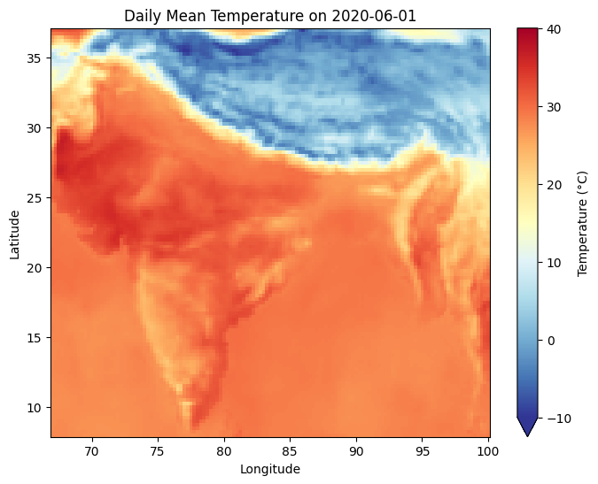
Creating an Animation of Temperature over June 2020
We will create an animation to visualize the change in daily mean temperature over the month of June 2020.
from matplotlib.animation import FuncAnimation
from IPython.display import HTML

# Create figure and axis
fig, ax = plt.subplots(figsize=(8, 6))

# Get the list of days in June
days = june_daily_mean_celsius.time.values

# Initialize the plot
data = june_daily_mean_celsius.isel(time=0)
img = ax.pcolormesh(
    data.lon, data.lat, data,
    cmap='RdYlBu_r', vmin=-10, vmax=40
)
plt.colorbar(img, ax=ax, label='Temperature (°C)')
ax.set_title(f'Daily Mean Temperature on {str(days[0])[:10]}')
ax.set_xlabel('Longitude')
ax.set_ylabel('Latitude')

# Update function for the animation
def update(frame):
    ax.clear()
    data = june_daily_mean_celsius.isel(time=frame)
    img = ax.pcolormesh(
        data.lon, data.lat, data,
        cmap='RdYlBu_r', vmin=-10, vmax=40
    )
    ax.set_title(f'Daily Mean Temperature on {str(days[frame])[:10]}')
    ax.set_xlabel('Longitude')
    ax.set_ylabel('Latitude')
    return img,

# Create the animation
anim = FuncAnimation(
    fig, update, frames=len(days),
    interval=200, blit=False
)

# Display the animation
HTML(anim.to_jshtml())Conclusion
In this tutorial, we explored the use of STAC, COGs, and Zarr to handle geospatial data efficiently. We demonstrated how to parse a STAC catalog, read Zarr data, and visualize temperature data over India during the Kharif season. This approach provides a scalable and efficient way to handle large geospatial datasets in cloud environments.